Derivatives – Sam Artigliere's Blog

Definition

A differential gives the slope of a curve (or function) at a specific point. This slope can be found by measuring the slope of a line tangent to the curve at that point. It can also be thought of as a measure of the change in the value of one variable that occurs when the value of a second variable is changed slightly at a specific value of the second variable. This is all very vague so let me try to explain.

Derivation

Consider a person walking down a straight road at constant speed due east. If we plot the displacement of the person, from its starting point, versus time, we get a straight line:

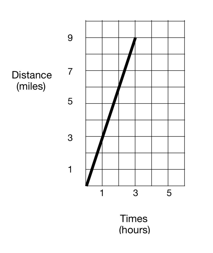
In figure 1, the distance traveled by the person is plotted on the vertical axis (ordinate), which we’ll call the y-axis. Time is plotted on the horizontal axis (abscissa), which we’ll call the x-axis. From the graph, we can see that, in the first hour, the person travels 3 miles (from 0 to 3 on the y-axis). In the second hour, it also travels 3 miles, from 3 to 6, and same with the third hour (the car travels from 6 to 9). So in this simple example, the speed of the car, obviously, is 3 miles/hour. This also is the slope of the linear plot of the car’s motion-rise over run; rise = 3, run = 1.

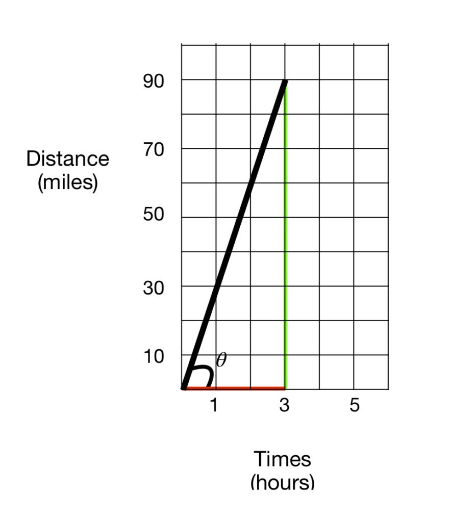
Suppose we drop a perpendicular from the end of the line that represents the car’s travel, point (3, 9), to the x-axis, at point (3,0). These 2 lines and the x-axis make a right triangle. The hypotenuse of the triangle and the x-axis make an angle, $\theta$ . The length of the perpendicular line (green line) and the length of the base of the triangle that runs along the x-axis (red line) equals $\tan \theta$ . Easy enough.

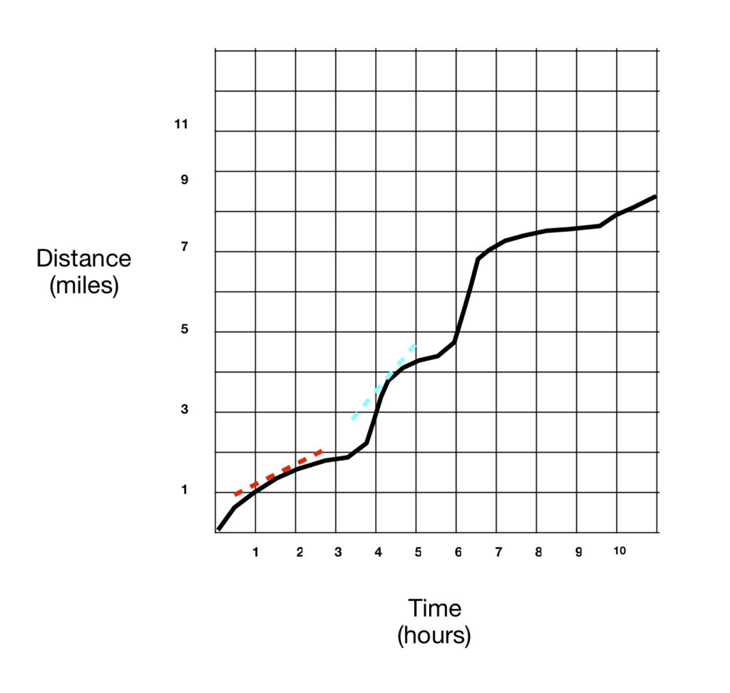
But what if we vary our speed, walking slowly some of the time and faster at others. A graph depicting our progress along the road might look something like figure 3. Suppose we want to know the speed of the car at 1.6 hours and 4.4 hours. How would we find it? Well, in the case of the straight line graph, the speed was given by slope of the line, which, as shown above, equals the tangent to the line. Perhaps this will work for the graph in figure 3 as well.

For example, the cyan dashed line is tangent to the curve at time = 4.4 hours. A tangent line, in turn, is a line that touches a curve at one point and is oriented in the same direction as the curve at that point. Because the tangent line and the curve are oriented in the same direction, their slopes must be the same. But how do we find such a tangent line.

We could start with trying to estimate the tangent line by picking a point on the curve, preferably close to the point of interest, and drawing a line between the 2 points. Such a line is called a secant line.

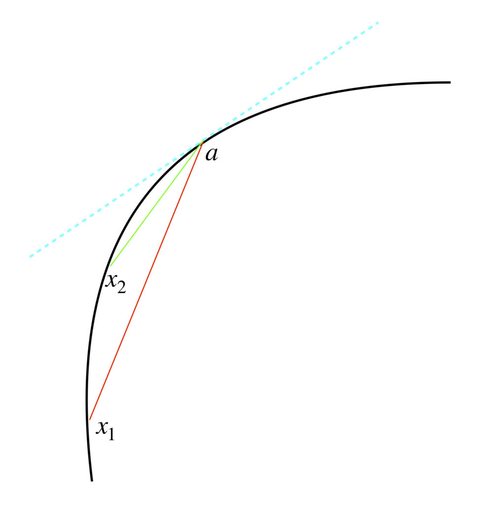
In figure 4, the red and green lines are secant lines; the dashed cyan line is a tangent line. $x_1$ , $x_2$ are the x-coordinates of the starting points of the red and green lines, respectively, and $a$ is the x-coordinate of both the endpoints of the red and green lines. The y-coordinates of the starting points of the red and green lines are $f(x_1)$ and $f(x_2)$ . $f(a)$ is the y-coordinate of the endpoint of the red and green lines. Just by eye, it’s clear that the shorter the secant line (i.e., the closer the x-coordinate of the secant line is to $a$ ), the closer is its angle of orientation to that of the tangent line. Specifically, the program used to draw figure 4 gives the angles of the 3 lines depicted. The dashed cyan (tangent) line is at $34^\circ$ , the red line is at $68^\circ$ and the green line is at $54^\circ$ .

If we keep making the starting point of the secant line closer and closer to point $a$ (and the secant line shorter and shorter) it will approximate the angle of orientation (and thus, the slope of) the tangent line better and better. This is shown in figure 5.

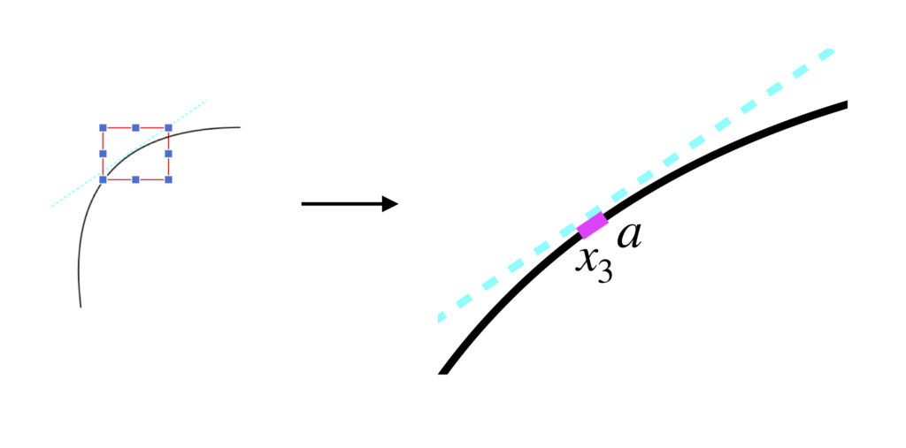
The diagram on the right-hand side of figure 5 is a blowup of the area where the tangent line touches the curve, $f(x)$ . The short purple line is a secant line. Notice that it is almost a straight line. Its angle is $34^\circ$ , so close to the angle of the tangent line that the drawing program is not accurate enough to detect a difference.

This little exercise suggests a general method for determining the slope of the tangent to a curve: namely, make the secant line smaller and smaller by taking starting points closer and closer to the point at which the tangent line touches the curve and see what slope value the slopes of those secant lines are tending toward. In mathematics, this process is called taking a limit. There is actually a formal mathematical definition for a limit. It can be found here.

Let me expound on how the limit can be used to find the derivative. The value of the slope of the secant lines is given by:

(1) $\begin{equation*}\frac{f(x)-f(a)}{x-a}\end{equation*}$

The process of taking the limit is written mathematically as:

(2) $\begin{equation*}\lim_{x\to a}\frac{f(x)-f(a)}{x-a}\end{equation*}$

Since this limit tells us what the slope of the curve is at the point, and as mentioned at the outset, the derivative of a curve at a point is the slope of the curve at that point, the expression in equation 2 is the definition of the derivative at that point.

One can define a general expression for the derivative of a function as follows:

Start at the point on the curve, $(x, f(x))$ . Move an infinitesimal distance, $h$ away from $(x, f(x))$ to point $(x+h, f(x+h))$ to form a secant line. Find the slope of this secant line:

$\begin{align*}\frac{f(x+h)-f(x)}{(x+h)-x}\end{align}$

(3) $\begin{equation*}\frac{f(x+h)-f(x)}{h}\end{equation*}$

To find the slope of the tangent line at $(x, f(x))$ , take the limit of equation 3:

(4) $\begin{equation*}\lim_{h\to 0}\frac{f(x+h)-f(x)}{h}\end{equation*}$

This, by definition, is the derivative of the function $f(x)$ .

There are a couple of different notations to indicate the derivative:

Leibnitz: $\frac{d\,f(x)}{dx}\text{ or }\frac{df}{dx}$
Newton: $f'(x)$