Table of Contents
- Preface
- I Introduction
- II Curvature
- III Einstein Field Equation
- IV Schwarzschild Metric
- V Confirmatory Evidence
Preface
These are some notes on general relativity. As in most of my pages, this is not meant to be comprehensive, but rather, to cover the basics and select topics that I feel I can better remember if I write them down.
As usual, explanatory notes can be accessed by clicking the appropriate link, often labeled “here.” To close the explanatory note, click the link again.
I. Introduction
Albert Einstein published his well-known paper on special relativity in 1905, a paper that described how lengths and time intervals vary depending on one’s frame of reference. However, this theory applies only to inertial frames of reference (i.e., frames of reference involving bodies that are at rest or moving at constant velocity). He wished to extend this theory to non-inertial (i.e., accelerating) frames.
I.A Equivalence Principle
His path to accomplishing this began in 1907 when, while sitting in his office in Bern, Switzerland, he had what he called “the happiest thought of [his] life.” He realized that a person in free fall from a rooftop does not feel his/her own weight and that objects that are falling with the person will continue to fall along side the person until they all hit the ground. The concepts embodied in this thought experiment are referred to as the equivalence principle and have been presented in several alternative forms over the years, most notably as an observer in an elevator that’s been dropped off a cliff, plummeting toward earth under the influence of gravity with an object (such as a ball) falling beside the observer. Such an arrangement is depicted in figure I.A.1.
In the diagram, we see an elevator in free fall with an observer and 2 red balls “floating” within it. We know from Newtonian physics that:
![\[ F=ma \quad \text{(I.A.1)} \]](https://www.samartigliere.com/wp-content/ql-cache/quicklatex.com-dbd40c9c4aeaa41cfbf99e9bb624aa71_l3.png "Rendered by QuickLaTeX.com")
where
 is the force on an object
 is the object’s mass, sometimes referred to as the inertial mass
 is the object’s acceleration
The force, in this case, is the force of gravity which, in Newtonian physics, is given by:
![\[ F = G\frac{mM}{r^2} \quad \text{(I.A.2)} \]](https://www.samartigliere.com/wp-content/ql-cache/quicklatex.com-27d97966905a80ae66853bf6862d1360_l3.png "Rendered by QuickLaTeX.com")
where
is the gravitational force between 2 objects
 is Newton’s gravitational constant =
and  are the masses of the object, sometimes referred to as the gravitational mass
Here, I use and for the masses in the Newton’s equation of gravitation because, in our example, I’ll let represent the mass of the earth and the mass of the smaller objects (i.e., the elevator, the observer, the balls).
Now we substitute eq. (I.A.2) into eq. (I.A.1). We get:
![\[ ma = G\frac{mM}{r^2} \quad \text{(I.A.3)} \]](https://www.samartigliere.com/wp-content/ql-cache/quicklatex.com-7b4e7d23671f8fad11bfb8ab7af4fe56_l3.png "Rendered by QuickLaTeX.com")
We can cancel on both sides. This gives us:
![\[ a = G\frac{M}{r^2} \quad \text{(I.A.4)} \]](https://www.samartigliere.com/wp-content/ql-cache/quicklatex.com-16ffdd9418d4165bd99be9fc21f22c54_l3.png "Rendered by QuickLaTeX.com")
Now let’s examine the units of the right side of eq. (I.A.4):
![\[ \frac{\cancel{L^3}}{\bcancel{M} \cdot T^2}\frac{\bcancel{M}}{\cancel{L^2}} = \frac{L}{T^2} = g \quad \text{(I.A.5)} \]](https://www.samartigliere.com/wp-content/ql-cache/quicklatex.com-251535abd471132449cd70e43fcf1912_l3.png "Rendered by QuickLaTeX.com")
Here,
is mass
 is length
 is time
We’re left with a term that has the units of acceleration, a term I’ve called  , the acceleration due to gravity. Thus, , the acceleration of the object affected by gravity equals the acceleration created by the gravitational force, . Note that these accelerations do not depend on the mass of the falling object, a well-known experimental result that legend has it Galileo established by dropping things from the leaning tower of Pisa. A basic principle we can extract from this little exercise is that inertial mass is equivalent to gravitational mass.
This seemingly simple idea has some profound consequences. First off, it explains why our observer in the elevator and objects next to them float weightlessly in the elevator as they fall: namely, because the frame of reference of the elevator is accelerating, and any observer in their own frame, don’t think they’re moving. Thus, over a sufficiently small region of spacetime, the frame of reference of an object in free fall is equivalent to an inertial frame of reference.
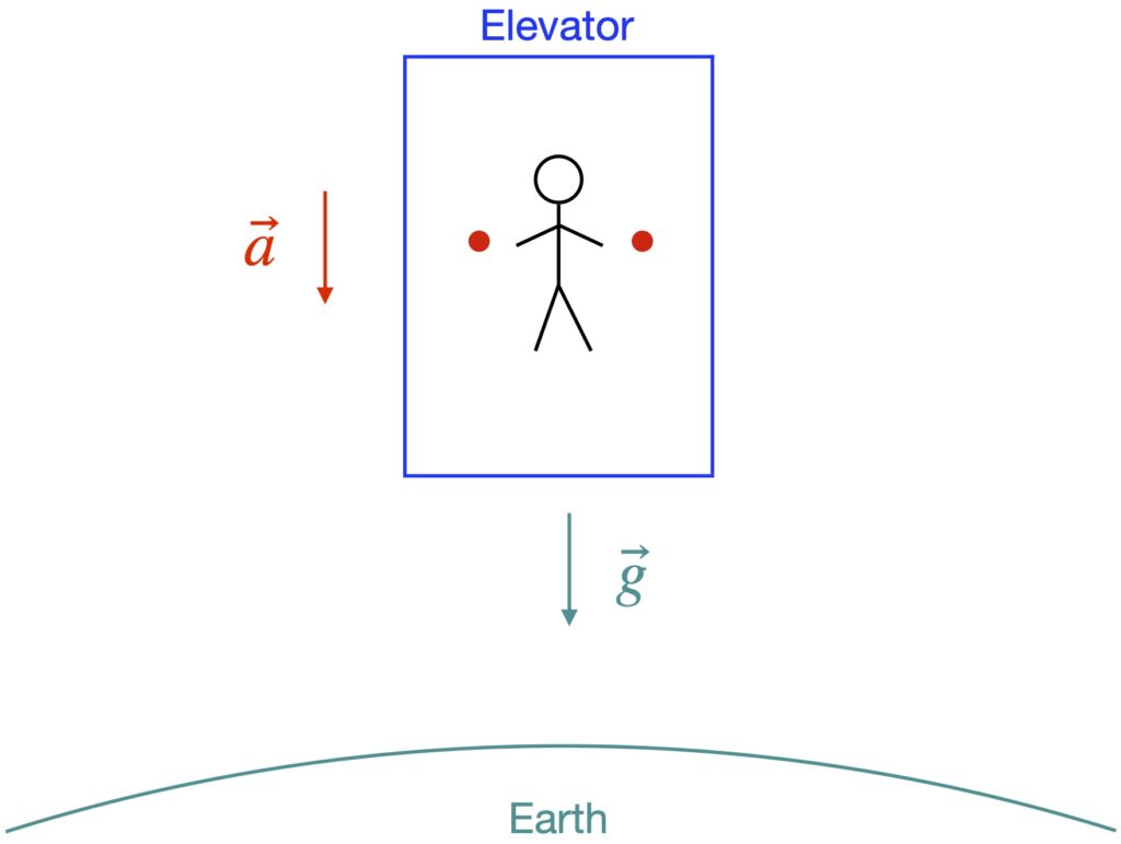
To see additional consequences of the equivalence of inertial and gravitational mass, let’s expand our thought experiment and imagine an observer in a rocket with a (red) ball at the rocket’s ceiling (figure I.A.2). Of course, if the rocket is moving at constant velocity (to an observer outside the rocket) or if the rocket is in free fall, the observer and the ball do not move. But now imagine that the rocket accelerates upward (relative to the observer in the rocket, to the ball in the rocket and to an observer outside the rocket) at 9.8 cm/sec, the acceleration known to occur due to the earth’s gravity . The observer outside the rocket sees 1) the rocket accelerating upward 2) the observer in the rocket plastered to the floor of the rocket and 3) the ball remaining at the same position while the floor of the rocket moves upward to meet it. By contrast, the observer in the rocket feels like he’s being pulled down against the floor of the rocket in a manner identical to being pulled down toward the earth while standing on the earth’s surface. In addition, the observer in the rocket sees the ball fall from the ceiling to the floor at a rate identical to the rate it would fall from the same height to the surface of the earth.
From this, we can conclude – like Einstein did – that acceleration and gravity are the same thing.
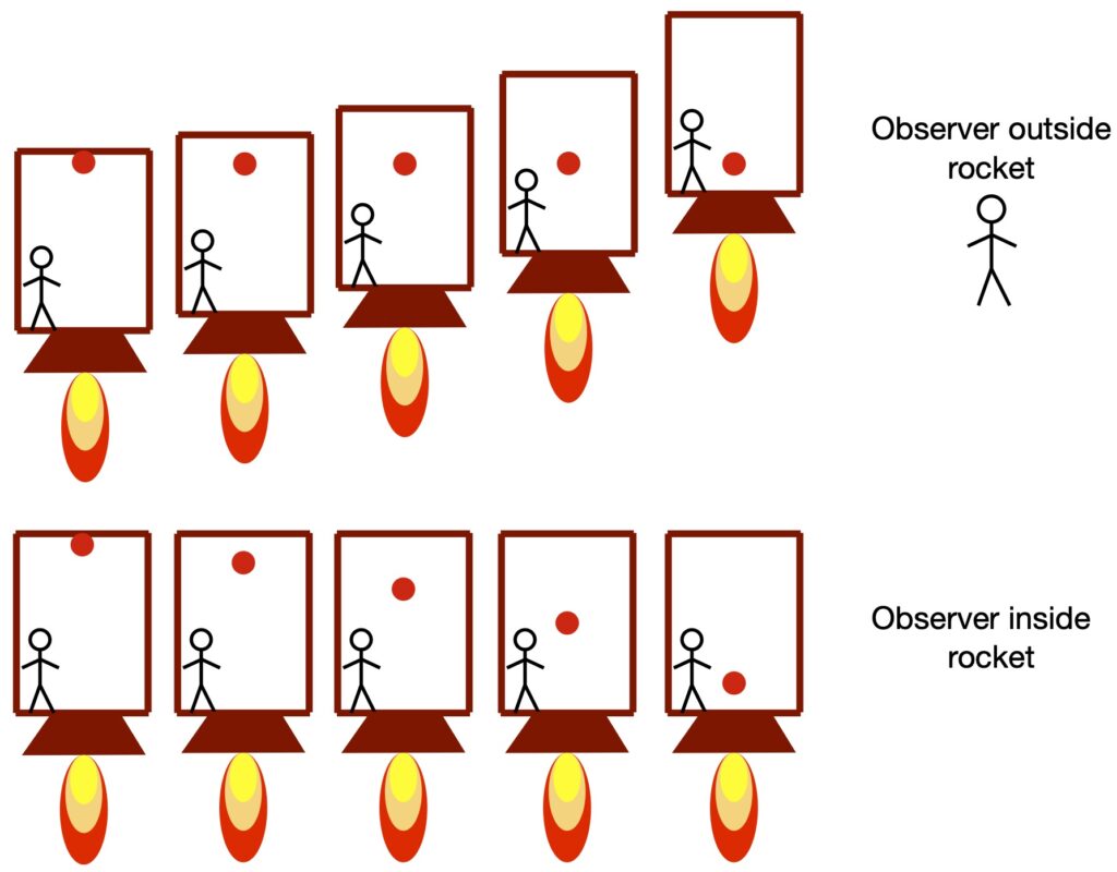
A similar phenomenon can be seen for light, as shown in figure I.A.3. In this figure, a light beam is shot in a rightward direction (let’s call it the x-direction) across an accelerating rocket. To an observer outside the rocket, the light beam appears to go straight across the rocket but the rocket’s floor gets increasingly close to the light beam as the rocket moves. On the other hand, an observer inside the rocket sees the light beam follow a parabolic path from the upper left to the lower righthand portion of the rocket. That is, the light gets “bent” in the accelerating frame of reference. And since Einstein considered acceleration and gravity to be equivalent, he concluded that gravity should “bend” light rays.
A more quantitative analysis of this problem yields further insight into what’s happening. In an inertial frame of reference, with the rocket moving in the z-direction with constant velocity,  , relative to an observer outside the rocket, we can write the following equations:


where the primed frame is that of an observer outside the rocket and the unprimed frame is that of an observer inside the rocket. Obviously, in special relativity, the expressions for spatial and time coordinate transformations would be more complex but this Newtonian view will suffice for our purposes here. We can also draw a spacetime diagram representing this inertial coordinate system, as in figure I.A.4.
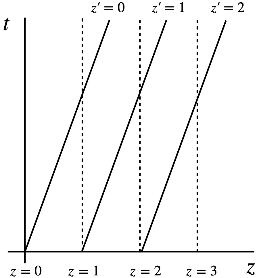
The dotted lines represent the worldlines of objects within the rocket from the point of view of an observer in the rocket. Such an observer doesn’t thing he’s moving in space, thus worldlines in this frame of reference are straight vertical lines (i.e., the observer inside the rocket sees himself and objects inside the rocket as moving in time but not space). By contrast, the observer outside the rocket sees the rocket and its contents moving in both space and time. Worldlines for this observer are depicted as diagonal solid lines. Again the lines are straight.
Now let’s write equations for the accelerating rocket. Specifically, we’ll write Galilean transformation equations relating the primed coordinates of an observer outside the rocket and the unprimed coordinates of an observer inside the rocket:

If we plot the primed coordinates on a spacetime diagram, we get something like this:
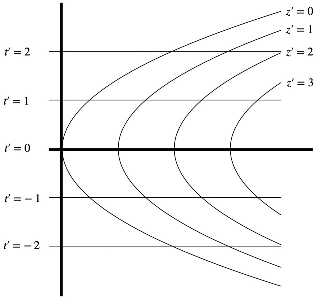
Instead of straight lines we get curved lines (i.e., parabolas) for the  coordinates.
Furthermore, we can write a transformation equation for the light ray in an accelerating elevator. In this case, an observer outside the rocket is stationary, in the z-direction, with respect to the light beam. This observer would write the following equations:


The observer in the elevator, however, is accelerating with respect to the light beam in the z-direction. Because of this relative acceleration, we’ll consider this observer’s coordinates to be the primed coordinates. This observer would write:


That means that:
![\[ t^2 = \frac{(x^{\prime})^2}{c^2} \quad \text{(I.A.9)} \]](https://www.samartigliere.com/wp-content/ql-cache/quicklatex.com-4f8b33d7836020a16d835390e6bf8a2b_l3.png "Rendered by QuickLaTeX.com")
Plugging eq. (I.A.9) into eq. (I.A.8), we obtain:
![\[ z^{\prime} = - \frac12 g \frac{(x^{\prime})^2}{c^2} \quad \text{(I.A.10)} \]](https://www.samartigliere.com/wp-content/ql-cache/quicklatex.com-3d3bf942d009fb00c315c137c0fc5c04_l3.png "Rendered by QuickLaTeX.com")
When we plot this equation, we get something like:
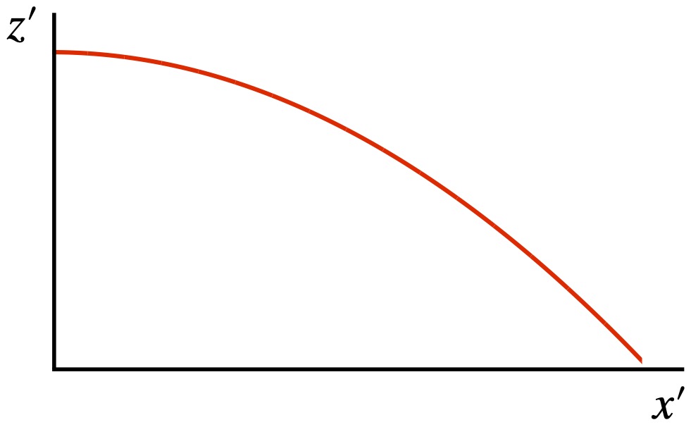
To Einstein, it was no coincidence that the path of light in an accelerated frame of reference and the coordinates in an accelerated frame are both curved in the same way (i.e., both are parabolas). Instead, it suggested to him that the light (or any other object for that matter) was simply following the shortest path along curved coordinates, coordinates that were the result of the acceleration. And because he presumed acceleration and gravity to be equivalent, he postulated that 1) gravity would also “bend” spacetime coordinates and 2) that light (and other objects) would follow these bent coordinates. Thus, it would appear that a massive object was exerting a gravitational force that was bending the light path (or the path of some other object), but really, the light (or the object) was just taking the shortest course it could along the bent coordinates. Such paths are referred to as geodesics; we will discuss them in greater detail later.
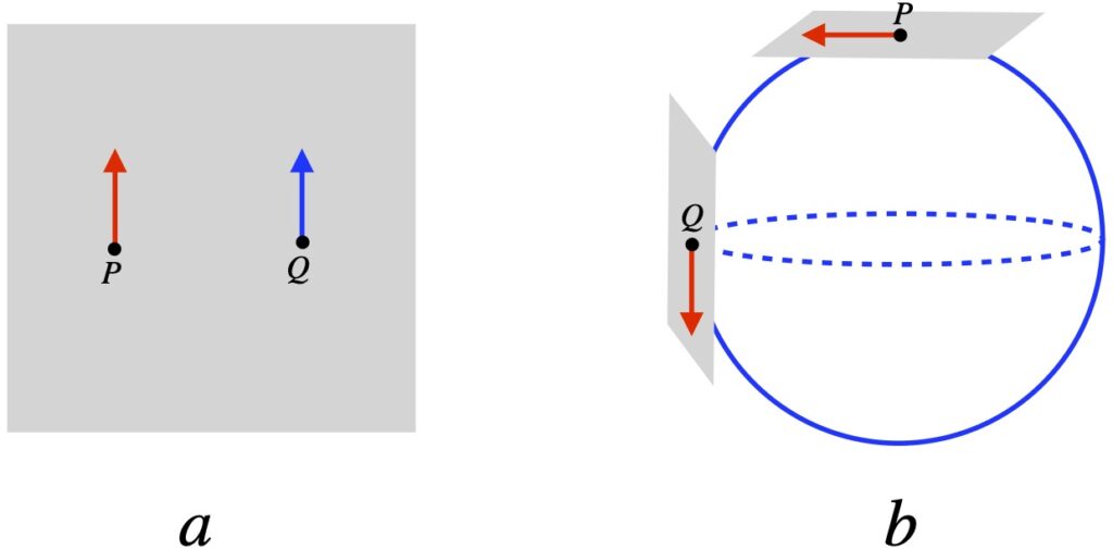
At any rate, Einstein developed these ideas further with another thought experiment. He imagined an observer (let’s call her observer A) at the center of a disc and another observer, observer B, at the outside of the disc. Across the diameter of the disc, we lay measuring rods. Let’s say it takes 10 of them to span the diameter of the disc. We also lay measuring rods around the circumference of the disc with the disc at rest with respect to the 2 observers. It takes 31.4 measuring rods to span the circumference of the disc.
Now we set the disc rotating. Each observer, in their own frame of reference – like any observer in their own frame of reference – sees themself at rest. However, observer A at the center of the rotating disc sees the observer B along the circumference of the disc as moving. From the theory of special relativity, we know that, to observer A, the measuring rods on the circumference of the disc undergo length contraction. Thus, it takes more than 31.4 measuring rods to span the circumference of the disc when the disc is in rotating motion relative to observer A. I don’t believe Einstein actually discussed this – in the context of this thought experiment – but per the theory of special relativity, to observer A, a clock on the circumference of the disc should tick slower than a clock at the center of the disc (i.e., time dilation takes place).
It has been noted that if such a disc were made of rigid material, it might break apart since, at each circumference level away from the disc center, differing degrees of circumferential length contraction should occur when the disc begins rotating while no length contraction should occur in the radial direction. Several solutions to this conundrum have been proposed in the literature such as, perhaps, the disc is made of malleable, fluid-like material or the disc is made of molten material which is allowed to cool only after the disc begins rotating. At any rate, this is a side argument that’s irrelevant to the point Einstein was trying to make.
Of course, observer B on the circumference of the rotating disc would also experience an outward (centrifugal) acceleration which would feel to him like gravity was pulling him outward. And since, in Einstein’s view, acceleration and gravity are equivalent, he reasoned that gravity should induce length contraction and time dilation as well.
So we have this idea that gravity has something to do with spacetime geometry with balls and light rays following curved paths that resemble the curved worldlines one sees with accelerated reference frames. And we also have this notion that gravity appears to cause length contraction and time dilation. If you’re like I was, you may be wondering, What’s the link between length contraction/time dilation and curved spacetime. Figure 1.7 provides one way to visualize this relationship.
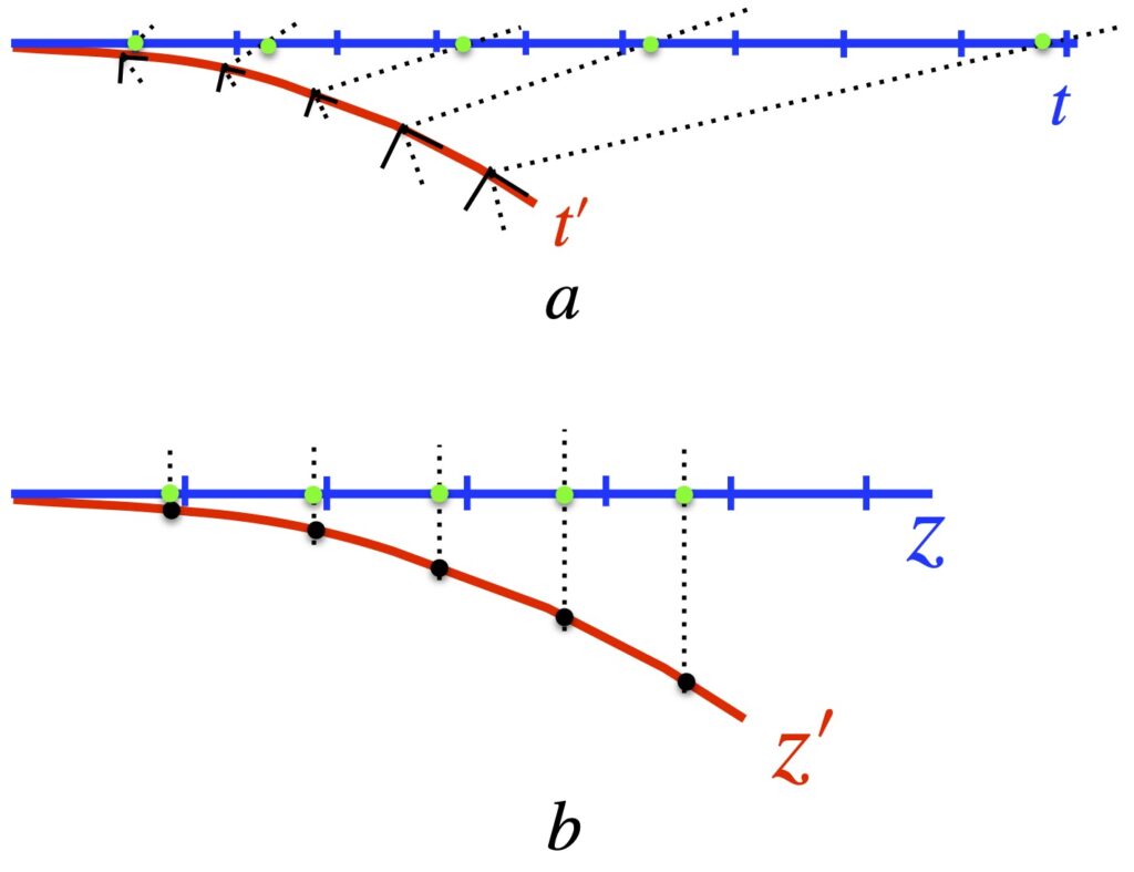
Figure I.A.7a, shows the time axes of 2 objects as seen by an observer very far away from a massive body. The blue time axis,  , is that of the far away observer, and thus, measures proper time for that observer. The red time axis,
  , corresponds to an object close to and moving toward the massive body, as seen by the far-away observer. An observer accompanying the object close to the massive body would – like any observer in their own frame of reference – think they aren’t moving. To this observer, each point in spacetime has, associated with it, a small set of coordinate axis which looks like flat (Minkowski) space (depicted in figure I.A.7a as little black axes at right angles to each other). The axes represent tiny local spacetime diagrams. The axis tangent to the red curve is the time axis. The axis perpendicular to the time axis is a spatial axis. In this setup, we’re only considering one spatial direction which we’ll call the z-axis. The dotted lines extending outward from the origin of each set of axes represent the path of light, oriented at 45°. The distance between the origin of each set of axes on the red time axis is equal to the tick marks on the blue axis, that distance representing 1 unit of time on both the blue and red axes. To see how the blue and red time axes relate to each other, an object moving along the red time axis sends out a light signal to the far-away observer from each set of axes, each pulse being – to the observer near the massive body – one time unit apart.
What time interval between these light pulses does the far-away observer detect? This is shown by the green dots at the intersection between the the path of the light rays (black dotted lines) and the blue time axis. What we see is that, as the object near the massive body gets closer to that body, the light signals it sends are detected by the far-away observer at time intervals that get farther and farther apart. If the path followed by the object close to the massive object had been straight, then the time intervals between light pulses would have been equally spaced, with length equal to the time intervals between the blue tick marks on the far-away observer’s time axis. Thus, we can see how time dilation can be thought of as a result of curved spacetime.
What about length contraction? This is addressed in figure 1.7b. In that figure, the blue axis (labeled  ) is the spatial axis of an observer far from a massive body. The red curved axis (labeled is the spatial axis of an object moving toward a massive body, as seen by the far-away observer. Of course, an observer moving with the object near the massive body – like any observer in their own frame of reference – thinks they’re not moving. They see space as flat and see the length interval between points on their spatial axis as being equidistant, each 1 length unit apart, the same length as the blue tick marks on the far-away observer’s (blue) spatial axis. To communicate his position to the far-away observer, the observer near the massive body sends a light signal from each black dot, to the far-away observer. The light moves in a straight line to the far-away observer, being received by the far-away observer, on the blue axis, at the green dots. Whereas the observer near the massive body measures the distance between each black dot as 1 length unit, the far away observer sees the units of length as being less than one unit, with that length interval decreasing as the object close to the massive body gets closer to that source of mass. That is, the far-away observer experiences length contraction. If the spatial axis in the frame of reference of the object near the massive body had been straight, then the black dots on that spatial axis would have coincided exactly with the blue tick marks on the blue axis. Therefore, we can see how length contraction can be thought of as the result of curved spacetime.
So we can see how Einstein’s thought experiment about objects in free fall that led to the simple idea that inertial mass equals gravitational mass got the ball rolling toward a theory – general relativity – that revolutionized scientific thought. Before we move on, we should note that this simple idea has a name – the equivalence principle – and that this principle has been expressed in 3 forms:
- Weak Equivalence Principle: Over sufficiently small spacetime regions, the motion of freely falling objects due to gravity cannot be distinguished from uniform acceleration.
- Einstein Equivalence Principle: In sufficiently small regions of spacetime, we. can find a representation such that the laws of physics reduce to those of special relativity.
- Strong Equivalence Principle: Gravity is ultimately a form of energy, and as such, behaves like mass in a gravitational field.
We won’t talk much about the strong equivalence principle in this article. We’ve already discussed the weak equivalence principle in some detail . At this point, we need to say a few words about the Einstein equivalence principle, mainly because it will be a good lead-in to our next section.
To illustrate the Einstein equivalence principle, consider the rocket ship containing an observer and a ball we talked about earlier. If the observer and ball took on a frame of reference where they accelerated with same constant acceleration as the rocket, then the observer would no longer be plastered to the floor of the rocket and the ball would no longer fall. They would float weightlessly in the rocket like an observer and a ball in a rocket in inertial motion (relative to some observer watching both rockets) in far outer space, far away from any massive objects. We know the spacetime in such an inertial frame of reference is the spacetime of general relativity – Minkowski space. And because the observer and ball in the uniformly accelerating frame behave like the observer and ball and rocket in outer space, we can surmise that the spacetime governing the uniformly accelerating frame is also that of special relativity. Thus, a coordinate transformation has been found that has changed things from a uniformly accelerating frame with behavior that looks like motion due to gravity to one with behavior that looks like special relativity.
Another way of thinking about this is to consider the earth whose surface is spherical – clearly curved. However, if we look at a small patch of the earth, it looks flat to us. Similarly, in curved spacetime (like spacetime axes in the region of a massive object), if we examine a small enough region, it will look flat (analogous to the flat coordinate system of special relativity). For those who are interested, I’ll offer a detailed proof of this but I’ll have to defer this proof until I’ve introduced Christoffel symbols.
I.B Tidal Forces
At any rate, we keep saying that acceleration equals gravity and the laws of physics are equivalent to general relativity (which occurs in flat Minkowski space) “in sufficiently small regions of spacetime.” This is because, over larger areas where gravitational effects are in play, this is not true. These are called tidal effects (or tidal forces) and they will ultimately allow us to differentiate accelerated motion in flat space from accelerated motion due to gravity.
Renowned physicist Leonard Susskind, in his lecture series and book on general relativity, illustrates these effects by an example that he calls the 2000 mile man.
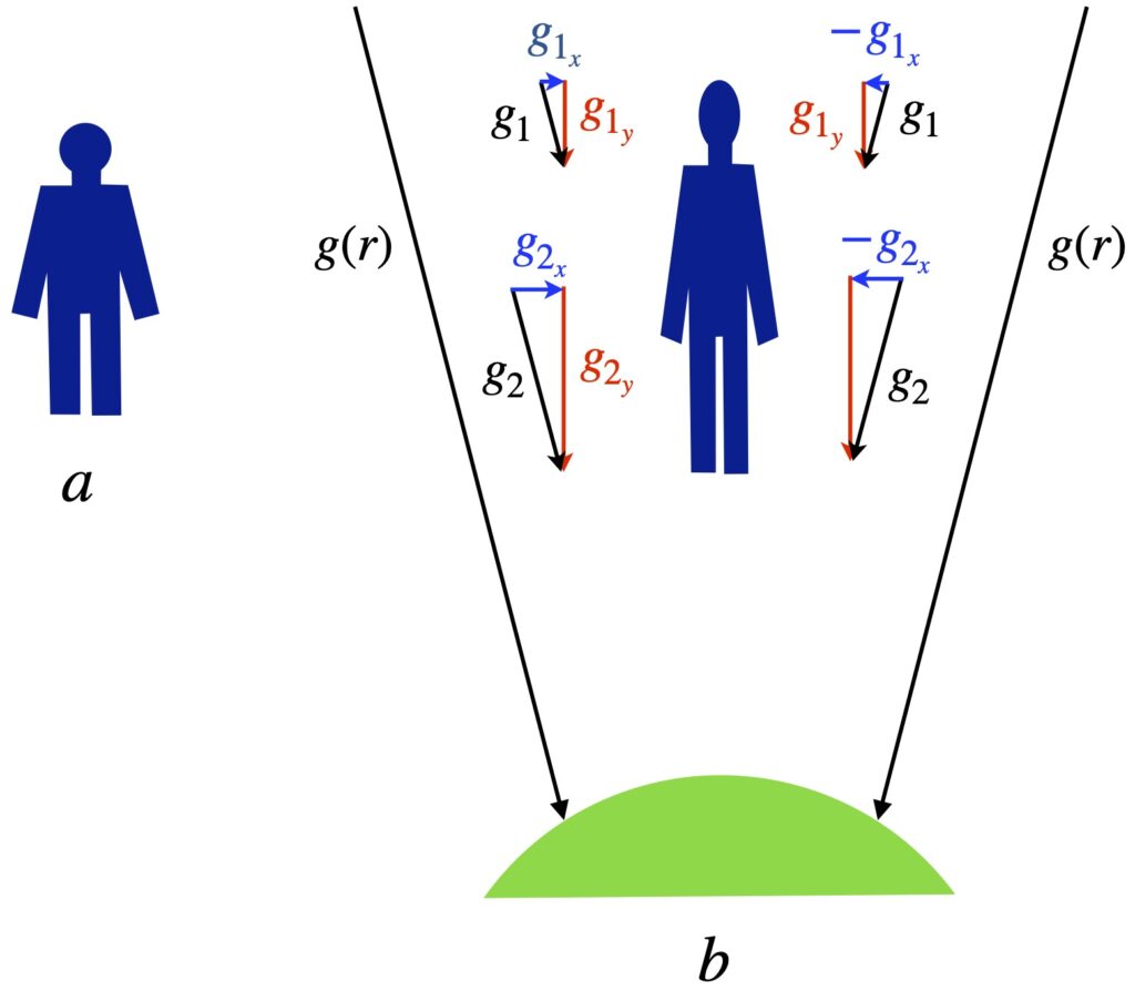
Figure 1.8a shows the 2000-mile-long man floating in space far from any massive body. Figure 1.8b shows the 2000-mile-long man near a massive body like the earth. Looking at things from a Newtonian point of view, the earth exerts a gravitational force,  , on the man – a force that’s a function of the distance from the center of the earth.
This gravitational force is oriented at an angle with respect to the long axis of the man. Thus, the man feels 2 components of force: one downward along his long axis and another directed inward toward his center. The latter inwardly directed forces squeeze him together. Meanwhile, the longitudinal forces vary from head to foot, the man experiencing a higher gravitational force near his feet (nearer the center of the earth) than at his head. This relative difference in longitudinal forces causes the man to stretch in the longitudinal direction.
When an accelerating frame of reference causes what appears to be a gravitational effect, we can always find a global coordinate transformation (i.e., a Lorentz transformation if we’re working in special relativity) that “gets rid” of the effects of gravity leading to a spacetime that looks flat.
On the other hand, this is impossible in a real gravitational field like that shown in figure 1.8. Why? Because the the gravitational field varies as a function of position, and thus, acceleration varies with position. If we try to make a global coordinate transformation that gets rid of the gravitational effect at one place (e.g., at the head of the 2000 mile man) then it won’t get rid of the gravitational effect in another place (e.g., at the feet of the 2000 mile man).
An even more extreme example would be to consider a person standing on the earth in Seville, Spain and another in Aukland, New Zealand, 2 locations separated by a straight line through the center of the earth. Both are influenced by earth’s gravity, but in opposite directions. Thus, if we make a global coordinate transformation that gets rid of the gravitational effect in Seville, it will double the gravitational effect in Aukland, and vice versa.
Einstein realized that frames of reference where there is no gravitational acceleration are equivalent to inertial frames of reference like the Minkowski space of special relativity, which we know is flat. By contrast, frames of reference where there is gravitational acceleration are associated with curved spacetime. We’ll defer proof of this until we acquire some additional mathematical tools, but for now, suffice it to say that we can always find a local coordinate transformation that makes a small region of curved spacetime flat. However, we can never identify a global coordinate transformation to make all of curved spacetime flat (proof ), and this inability to find such a global coordinate transformation is what tells us that a true gravitational effect (not just acceleration in flat space) and, thus, curved spacetime, is present.
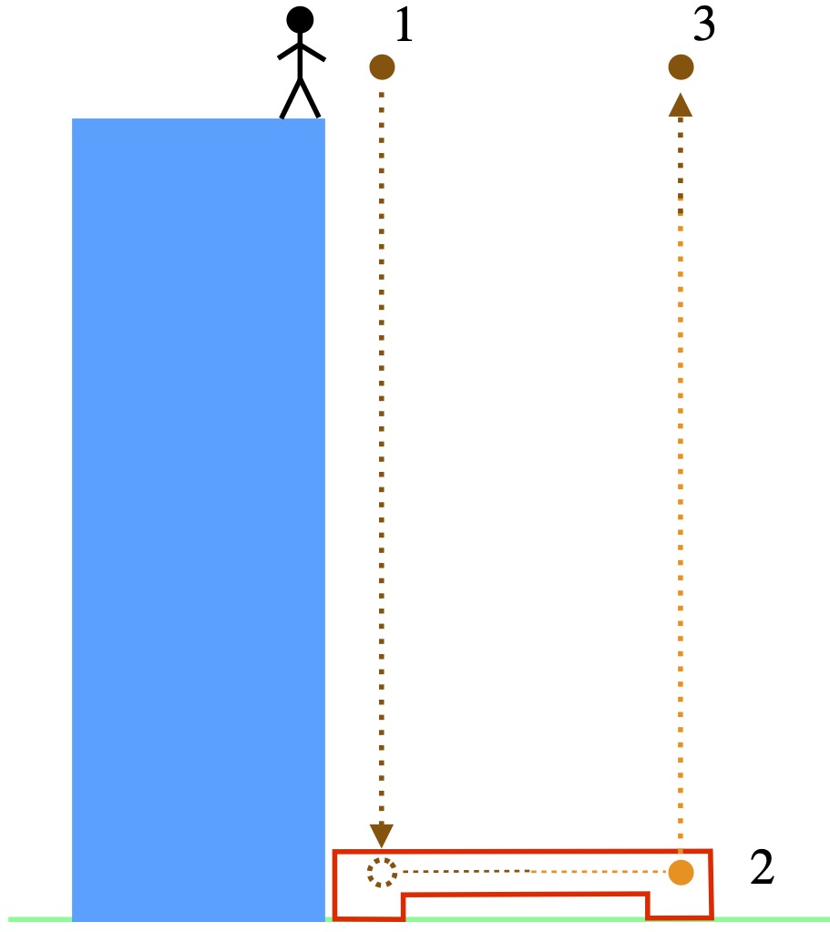
 where
where  . Thus, the initial energy of the rock before it’s dropped is just
  where
where  . The photonulator has perfect efficiency so the photon’s energy initial energy is equal to the rock’s total energy:
 where
where is the total energy at the bottom of the experimental setup (i.e., ground)
 is the reduced Planck’s constant
 is the frequency of the photon on the ground
 , is measured again at the same level as that from which it was initially dropped. What is its energy? Well, if we believe in the law of conservation of energy,
 ![\[ \frac{E_T}{E_B} = \frac{m}{m(1 + gh)} = \frac{\omega_T}{\omega_B}\quad \Rightarrow \quad \omega_T = (1-gh) \omega_B \]](https://www.samartigliere.com/wp-content/ql-cache/quicklatex.com-c906f272651fd514f6285675a410a377_l3.png "Rendered by QuickLaTeX.com")
 . This makes sense since 1) the energy of the photon at the top of the tower should be lower that the energy of the photon at the bottom of the tower (i.e., by the time it gets back to the top, it had to have “lost back” the energy the rock gained by falling to the ground) and 2) a lower energy means lower frequency.
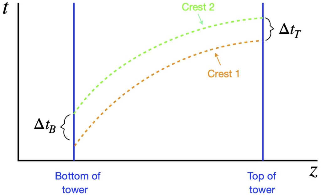
 , and this time separation should be maintained along the entire worldlines of crest 1 and crest 2. In other words:
 ![\[\Delta T_B = \Delta T_T\]](https://www.samartigliere.com/wp-content/ql-cache/quicklatex.com-7dc6b0e3374594e95dba027472bc2d63_l3.png "Rendered by QuickLaTeX.com")
![\[ \Delta T = \frac{2\pi}{\omega} \]](https://www.samartigliere.com/wp-content/ql-cache/quicklatex.com-99768cbbe97b0c88e82ddc6053f8e6f2_l3.png "Rendered by QuickLaTeX.com")
![\[ \Delta T_B = \Delta T_T = \frac{2\pi}{\omega_B} = \frac{2\pi}{\omega_T} \]](https://www.samartigliere.com/wp-content/ql-cache/quicklatex.com-ca4de92439966bc360a3bb57662c0c12_l3.png "Rendered by QuickLaTeX.com")
How, then, can one determine whether true gravity/curved spacetime or acceleration in flat spacetime exists? Testing all possible coordinate transformations by trial and error could give us the answers but this, of course, is impractical. Einstein realized that he needed some novel method to make the differentiation. For this task, he turned to mathematician colleagues like Marcel Grossman who helped him find such a method: differential geometry. We’ll see how this helped to solve Einstein’s dilemma in the next section.
Curvature
Everything we do in this section is geared toward developing a mathematical method of differentiating flat spacetime from curved spacetime. However, this will involve several steps. To understand this process, the reader will need a basic understanding of tensors and Einstein summation notation. For those readers who need to learn about these topics, I have a tensors page on this website that gives an introduction to these subjects. There are several more comprehensive treatments on these topics elsewhere on the web. I list a few references to such sites in my tensors page. I’ll only provide an introduction to several of the topics I discuss in my tensor page but go into depth on topics I haven’t covered elsewhere.
II.A Metric Tensor
We talked previously about Einstein’s thought experiment involving the rotating disc which showed how accelerating frames of reference, and thus gravity, can give rise to time dilation and length contraction. We then discussed how the variability in the magnitude of time and spatial units is related to curved spacetime. The metric tensor is what tells us the lengths of line elements, and therefore, the magnitude of the time and spatial units in spacetime.
Specifically, the length of a vector is given by the dot product with itself:


Suppose we have an infinitesimal displacement vector  . To find its length,
  , we take the dot product with itself:


To get the length, , we take the square root of eq. (II.A.2).
Notice that, in eq. (2.1.2), we’ve defined the entity 
where, if we’re working in 2 dimensions,  could be expressed as a matrix:

As it applies to physics, we can imagine that a tiny coordinate axis exists at every point in spacetime and that a metric exists at each point where the metric gives the relative lengths of the basis vectors in these infinitesimal coordinate systems. In flat spacetime, the metric is the same everywhere. An example is the spacetime of special relativity, Minkowski space, where the metric is the same at every point and is given by:
![\[ \eta = \begin{bmatrix} -1&0&0&0 \\ 0&1&0&0 \\ 0&0&1&0 \\ 0&0&0&1 \end{bmatrix} \quad \text{or} \quad \begin{bmatrix} 1&0&0&0 \\ 0&-1&0&0 \\ 0&0&-1&0 \\ 0&0&0&-1 \end{bmatrix} \quad \text{eq. (II.A.4)} \]](https://www.samartigliere.com/wp-content/ql-cache/quicklatex.com-26cd87b51660f0493fd32a74f71ee90f_l3.png "Rendered by QuickLaTeX.com")
In curved spacetime, this is not the case. The metric varies from point to point. This might cause one to wonder, Is calculation of the metric a way to check to see if spacetime is flat? (i.e., if the metric is the same everywhere, the space is flat; if not, it isn’t). It turns out that we can always find a set of coordinates where  and
and  (i.e., where the metric is not changing to first order. However, if the space is curved, we can never find a coordinate system where
  . A proof of this can be found :
 be our starting coordinate system with metric
 be coordinates in which spacetime has a Lorentz representation in the vicinity of some event (i.e, spacetime point)
 ![\[P \doteq \{x^{\mu}_P\} \doteq \{x^{\bar{\mu}}_P\} \quad \text{(1)} \]](https://www.samartigliere.com/wp-content/ql-cache/quicklatex.com-076a6e36369f9a96c0f8fa2c7390238b_l3.png "Rendered by QuickLaTeX.com")

 .
.![\[ g_{\bar{\mu} \bar{\nu}} = L^{\alpha}_{\bar{\mu}} L^{\alpha}_{\bar{\nu}} g_{\alpha \beta} = \eta_{\bar{\mu} \bar{\nu}} \quad \text{(2)} \]](https://www.samartigliere.com/wp-content/ql-cache/quicklatex.com-055999150121148f9340b7257cd2a907_l3.png "Rendered by QuickLaTeX.com")
 in a Taylor series and manipulate it. Our strategy will be to compare the degrees of freedom offered by the coordinate transformation (which we can select) to the constraints imposed by the metric and its derivatives (which we’re given).

 ,
,  and
and  terms are given to us and provide the constraints.
 ,
,  and
and  terms are freely specifiable and provide us with degrees of freedom we can use to satisfy the constraints.
![+ (x^{\bar{\gamma}} - x^{\bar{\gamma}}_P)\bigl[ 1^{rst} \text{ deriv. terms} \bigr] \quad 1^{rst} \text{ order}](https://www.samartigliere.com/wp-content/ql-cache/quicklatex.com-75c44268f1c0f7f7219bb92c829f91c8_l3.png "Rendered by QuickLaTeX.com")
![+ \frac12 (x^{\bar{\gamma}} - x^{\bar{\gamma}}_P)(x^{\bar{\delta}} - x^{\bar{\delta}}_P) \bigl[ 2^{nd} \text{ deriv. terms} \bigr] \quad 2^{nd} \text{ order}](https://www.samartigliere.com/wp-content/ql-cache/quicklatex.com-c2e80e959bd76853ba05bef0881e02d1_l3.png "Rendered by QuickLaTeX.com")

 order:
 is a nonsymmetric 4 x 4 matrix, meaning that all 16 elements constitute degrees of freedom.
 to make
  at
at  order:
 gives us 10 constraints due to the symmetric 4 x 4 matrix.
  has 4 components leading to 4 constraints.
 gives us 4 DOFs from
  and
and  terms form a symmetric 4 x 4 matrix leading to 10 DOFs.
 order:
 leads to 10 constraints emanating from the symmetric 4 x 4 matrix created by the
  . We get 4 DOFs from the
  ,
,  terms form a symmetric 4 x 4 x 4 matrix. The number of DOFs engendered by these terms requires some combinatorics:
![\[ \eval{\frac{n(n+1)(n+2)}{3!}}_{n=4} = \frac{4 \cdot 5 \cdot 6}{6} = 20\]](https://www.samartigliere.com/wp-content/ql-cache/quicklatex.com-bbbae2d74f0597a9fce6949e47a520cd_l3.png "Rendered by QuickLaTeX.com")
![\[ g_{\bar{\mu} \bar{\nu}} = \eta_{\bar{\mu} \bar{\nu}} + \mathcal{O}[(\partial^2 g)(\delta x)^2 ] \quad \text{(6)} \]](https://www.samartigliere.com/wp-content/ql-cache/quicklatex.com-b15d486802a5a1fbdb4a9be11abd61b2_l3.png "Rendered by QuickLaTeX.com")
 and have 20 independent components which make up the additional 20 DOFs we were missing after the above derivation.
 .
.Thus, we can’t use the metric alone to determine whether or not a space is flat. As we’ll see later, to do this, we’ll have to come up with a mathematic object that incorporates the second derivative of the metric.
There are a few properties of the metric that we should briefly mention here:
- The metric tensor is a symmetric tensor.
- The covariant derivative of the metric tensor is zero:
 .
. - The metric tensor can be used to raise and lower indices on tensors. For example:
 .
.
II.B Covariant Derivative
The first topic we need to touch upon on our way to understanding curvature is the covariant derivative. Briefly, if we are working in Cartesian coordinates, we can take derivatives and partial derivative in the manner that’s taught in undergraduate calculus classes i.e., by taking the derivative of vector components. This works because, in Cartesian coordinates, basis vectors are the same everywhere. However, in non-Cartesian coordinates in flat spacetime (e.g., non-orthogonal axes, Minkowski spacetime), basis vectors are not constant. The problem is even more severe in curved spacetime where basis vectors vary from point to point. We want our derivative operation to return a tensor, because the laws of physics should be invariant in all frames of reference, and the only way that this can happen is if we use tensor equations to describe them. And the only way to return a tensor from our derivative operation is to take basis vectors into account.
Let’s look at a vector

where
 are the components of the vector
 are the basis vectors
If we want to take the derivative of this vector  , since both the components and basis vectors can vary, we need to use the chain rule:


The result, referred to as the covariant derivative, is a tensor.
II.C Christoffel Symbols
The righthand-most term in eq. II.B.2 is frequently expressed in the following way:

And so, eq. II.B.2 becomes:

Changing some indices and rearranging, we get:

The term in parentheses is called the covariant derivative:

It represents the component of the derivative of vector  in the
  direction and – as opposed to Christoffel symbols alone – it is a tensor.
The meaning of the Christoffel symbol is shown in figure II.C.1.
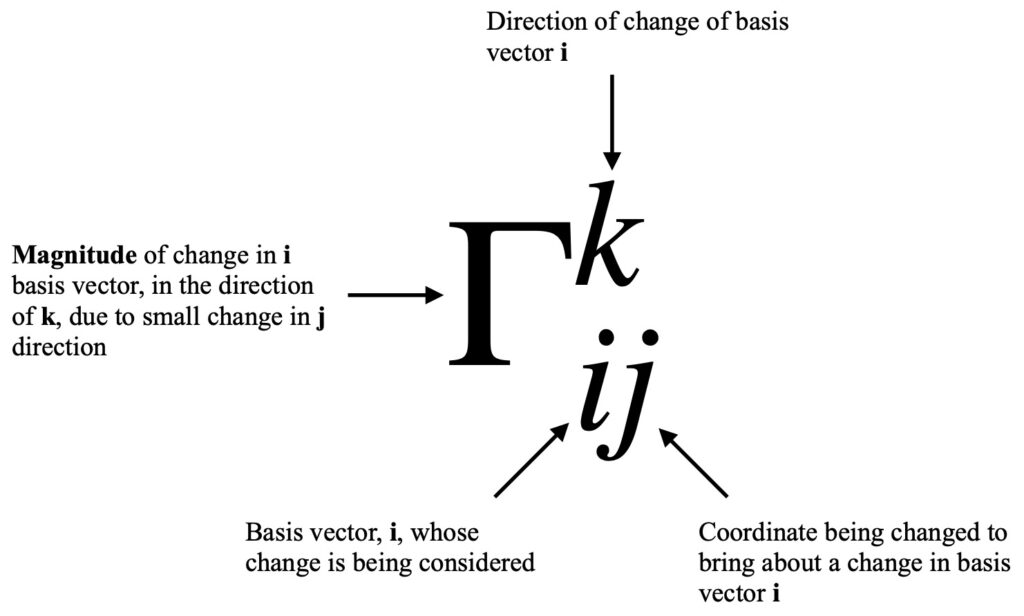
There are 2 types of Christoffel symbols, depending on how they’re expressed in terms of the metric. Christoffel symbols of the first type are written as:
![\Gamma_{lij}=\displaystyle \frac12 \left[\displaystyle \frac{\partial g_{li}}{\partial x^j} + \frac{\partial g_{lj}}{\partial x^i} + \frac{\partial g_{ij}}{\partial x^l}\right] \quad \text{eq (II.C.5)}](https://www.samartigliere.com/wp-content/ql-cache/quicklatex.com-1b6f0993127c4378522ed5c5f998a87d_l3.png "Rendered by QuickLaTeX.com")
Christoffel symbols of the second type are written as:
![\Gamma^l_{ij}=\displaystyle \frac12 g^{kl}\left[\frac{\partial g_{ik}}{\partial x^j} + \frac{\partial g_{jk}}{\partial x^i} - \frac{\partial g_{ij}}{\partial x^k}\right] \quad \text{eq (II.C.6)}](https://www.samartigliere.com/wp-content/ql-cache/quicklatex.com-d41b904fb5ba99c2932ba050618c7323_l3.png "Rendered by QuickLaTeX.com")
Derivations of eq. (II.C.6) can be found here:
It’s the Christoffel symbols of the second type, the one most often used in general relativity, that we’ll be using in this article.
It should be noted that the Christoffel symbol is a kind of connection coefficient. There are many ways we can define connection coefficients. The Christoffel symbol of the second type, as defined above, is also called the Levi-Civita connection.
II.D Parallel Transport
We would expect that, to take the covariant derivative in a curved space, we could simply take the difference between 2 vectors,  and
and  , separated by a short distance,
  , then take the limit as goes to zero:

However, we can’t do this because  is undefined. This is due to the fact that, in order to compare 2 vectors, they have to be in the same tangent plane. But the tangent spaces at points P and Q in a curved space are not the same, as shown in figure II.D.1.
We can show this algebraically as well. We know we can express vectors as a sum of components and basis vectors:

In flat space, we can write the quantity as:

Because, in flat space, the tangent space and basis vectors are the same everywhere, we have  . Therefore:

and we can subtract components in the numerator of our expression for the derivative in eq. (II.D.1).
However, if coordinates are curved, basis vectors (and in the case of curved space, tangent planes) aren’t the same at the points P and Q. Thus, we can’t just subtract components in the numerator of the expression for the derivative.
In order to compare 2 vectors in curved space, we need to transport one vector to the tangent space of the other vector, then compare them. How do we transport them? By a process called parallel transport.
What does it mean to parallel transport a vector? In words, it means “as we progress along a path (e.g., worldline or coordinate line), keep the vector parallel to itself.” This translates, in mathematical terms, to “the covariant derivative of the vector, in the direction of the tangent vector, is zero” which means that, when we move along the tangent vector (i.e., move along a worldline or other parameterized curve because the tangent vector is everywhere parallel to the curve), the vector does not change. The equation that expresses this idea is:

where

In pictorial form:
In figure II.D.2a, we see parallel transport in flat space. The vector just points in the same direction at every point along a closed loop and it ends up pointing in the same direction that it started at the apex of the loop.
In figure II.D.2b, we see parallel transport in a curved space, the surface of a sphere. The way we can visual this is to imagine that the vector we’re parallel transporting is a spear being held by a person walking along the curve. He starts at the top of the closed curve and walks along the curve with the spear pointing along the direction he’s walking. When he reaches the equator, the curve he is traversing courses to the right. In an attempt to keep the spear pointing in the same direction, the person keeps the spear pointing down (the same direction it was pointing when it reached the equator). To do this, he walks sideways and rightward. At the point where the curve courses upward from the equator, again, keeping the spear pointing down, the person carrying the spear keeps it pointing down but walks backward. As he walks backward, the spear remains in the tangent plane but the tangent plane gets “tilted backward” as he walks. When he reaches the starting point, at the apex of the curve, the spear (i.e., the orange vector) remains in the tangent plane (as it does all along the curve) except that it points in a direction different from that in which it pointed at the start of its journey (green vector). Thus, despite “trying to keep the spear (vector) parallel” as it was transported around the closed loop, when it reaches the origin of the trip, the spear (vector) points in a different direction that in which it started because the direction of the basis vectors changed as the curve was traversed.
I go through this little exercise here because parallel transport will play a central role in understanding geodesics and the Riemann tensor, the ultimate tool we’ll us to determine spacetime curvature.
II.E Lie Derivative
Lie transport is an alternative way to look at transporting vectors and gives rise to the Lie derivative, Lie bracket, Killing vector fields and spacetime symmetries. While these topics are useful for advanced applications in general relativity, they aren’t immediately important for what I’m covering in this article. However, in my first go-round in learning general relativity, I admit I was befuddled by Lie derivatives and their associated topics so I’ve decided to discuss them here, largely to enhance my own understanding. Because they are a bit of an aside, I’ll provide links which can be clicked to see the information on these subjects, if the reader so desires.
II.E.1 Derivation
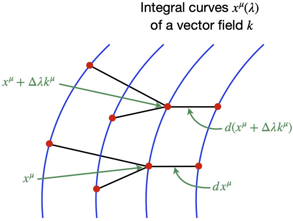
In the covariant derivative, we use parallel transport to transport one vector to another so they can be compared. The mathematical object that facilitates this transport is the Christoffel symbol which is a function of the metric. But there are other ways to transport vectors so they can be compared. One is Lie transport. A vector undergoing Lie transport follows the “flow” of integral curves created by a vector field. The comparison it allows is called the Lie derivative. Figure 1 depicts Lie transport along integral curves and defines the quantities we will need to find the Lie derivative.
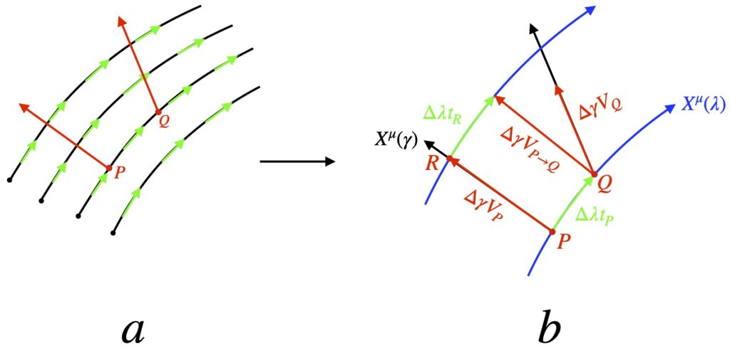
As shown in figure 1a, we start with a vector field with tangent vectors (shown in green) that can be connected to constitute integral curves (also called flow lines). Figure 1b shows a small section of the vector field noted in figure 1a with tangent vectors (green), , along 2 integral curves (blue) parameterized by a variable  with coordinates
  .
.
We define a displacement vector, oriented along an integral curve parameterized by the variable  , pointing in a direction defined by coordinates
  , with tangent vector
  . The displacement vector extends from point P to point R, point R lying along one of vector field flow lines. Its length is
  (which is what we’ll call this vector).
We define another displacement vector along another flow line of vector field  with tangent vector
  . This displacement vector starts at point Q and has length
  so we’ll call it .
We define a third displacement vector from point P to point Q along the tangent vector between the 2 points,  . Its length is and we’ll call it
  .
.
Finally, we construct a fourth displacement vector along the upper flow line, beginning at point R and extending a distance along the tangent vector,  , on that flow line. We’ll call this displacement vector
  .
.
We now transport vector to point Q, dragging its base along to point Q, its tip ending up at the tip of . This is called Lie transport. We’ll call this transported vector  .
.
Now we subtract  from to get the Lie derivative.
Let’s make this a bit more mathematically precise.
First, , the tangent vectors along the and  flow lines can be expressed as a differential operator:

The components of are:

That means that:

Now we define the Lie derivative as:

where, for the time being, we’ll use  to refer to the Lie derivative.
Next, we multiply both sides of eq. (4) by  . We get:

We know that we the components of a displacement vector are just the difference between its coordinates at its tip and its tail. So:


Let’s look at the  component of eq. (5):

Let’s examine the term  and
and  :
:


and


We put the results of eq. (8) and eq. (9) back into eq. (7) and obtain:
![\displaystyle \Delta \gamma \frac{"dV"}{d \lambda} = \lim_{\Delta \lambda \rightarrow 0} \frac{1}{\Delta \lambda} \Bigl[ \Delta \gamma V_Q^{\mu} - (\Delta \gamma V_P^{\mu} + \Delta \lambda t_R^{\mu} + \Delta \lambda t_P^{\mu}) \Bigl]](https://www.samartigliere.com/wp-content/ql-cache/quicklatex.com-2adcd760dc66af4e36db1ce1b6871cfb_l3.png "Rendered by QuickLaTeX.com")

![+ \Delta \lambda(t^{\mu}_P + \Delta \gamma V^{\alpha}_P \partial_{\alpha} t^{\mu}_P) - \Delta \lambda t_P^{\mu} \Bigr]](https://www.samartigliere.com/wp-content/ql-cache/quicklatex.com-9d255cf337ef8c154ae78d6869488ed9_l3.png "Rendered by QuickLaTeX.com")

![- \bcancel{\Delta \lambda t^{\mu}_P} - \Delta \lambda \Delta \gamma V^{\alpha}_P \partial_{\alpha} t^{\mu}_P) + \bcancel{\Delta \lambda t_P^{\mu}} \Bigr]](https://www.samartigliere.com/wp-content/ql-cache/quicklatex.com-debf50132d72c4665913d4144f6a679c_l3.png "Rendered by QuickLaTeX.com")
We can cancel ‘s and ‘s leaving us with:
![\displaystyle \cancel{\Delta \gamma} \frac{"dV"}{d \lambda} = \lim_{\Delta \lambda \rightarrow 0} \frac{1}{\bcancel{\Delta \lambda}} \Bigl[ \cancel{\Delta \gamma} \bcancel{\Delta \lambda} t^{\alpha}_P \partial_{\alpha} t^{\mu}_P - \bcancel{\Delta \lambda} \cancel{\Delta \gamma} V^{\alpha}_P \partial_{\alpha} t^{\mu}_P \Bigr]](https://www.samartigliere.com/wp-content/ql-cache/quicklatex.com-308c32d20dd8f51228368c7db9fbbc17_l3.png "Rendered by QuickLaTeX.com")
and ultimately:

In arriving at eq. (10), we drop the  subscripts since we’ve taken the limit as goes to zero meaning the points and
  essentially coincide.
The Lie derivative is usually denoted by  . So we have:

which denotes the component of the Lie derivative of with respect to .
II.E.2 Other Lie Derivatives
II.E.2.a Lie Derivative of a Scalar

II.E.2.a Lie Derivative of a (0,1) Tensor
We know that when a (0,1) tensor (i.e., a covector) acts on a vector, we get a scalar, so we have:

We know how the Lie derivative acts on a scalar, so we get:

Applying the product rule to the Lie derivative gives us:

We know how to take the Lie derivative of a vector i.e., a (1,0) tensor. Thus, eq. (14) becomes:

We expand the righthand side of eq. (13) using the product rule. This yields:

When we equate the righthand sides of eq. (15) and eq. (16), we obtain:


We want to cancel the term  on both sides. To do this, we rename dummy indices in the righthand term on the righthand side of eq. (18):


Doing this gives us:

After making these cancellations, we are left with:

II.E.2.c Lie Derivative of (n,m) Tensor
We can generalize the expression of the Lie derivative to tensors of any rank as follows:
Let  be a tensor of rank
  . Then the Lie derivative is:

III.E.3 Spacetime Symmetries
In figure X, we have integral curves,  (shown in blue) of a vector field
  . What we mean by spacetime symmetry is that all of the points along the flow lines of the vector field remain separated by the same spacetime distance. That means that, if there is spacetime symmetry, then the spacetime separations between the points separated by
  and
and  are equal. That is:

We expand each of the terms on the righthand side of eq. (2) in a Taylor series to first order:


All of the  terms raised to powers of
  are negligible and can be ignored. Thus, we have:


We can divide through by to obtain:


Next, we rename some dummy indices. Specifically, in the first term on the lefthand side, we change  ; in the second term on the lefthand side, change
  . That gives us:


This allows us to divide through by  . When we do this and rearrange, we are left with:

But we recognize eq. (6) as the Lie derivative of the metric along the vector field :

What this means is that spacetime is symmetric along the integral curves of a vector field if  . And the vector field that defines this symmetry is called a Killing vector field.
Now let’s examine an important consequence of these findings. Consider what happens if one of the coordinate basis vectors is a Killing vector field. Suppose, for example, that the  coordinate basis vectors are a Killing vector field. The basis vector along the flow lines that make up the field is given by
  . The fact that the field is a Killing vector field means that . Expanding this out, we get:

The Killing vector field consists of just the flow lines so we can say:

Because  is a constant, the terms in eq. (8) with
  in them become zero. The first term in eq. (8) becomes
This tells us that, if one of the metric components is independent of one of the coordinates (i.e., its derivative is zero which means it doesn’t change), then 1) the vector field that defines that coordinate is a Killing vector field and 2) the spacetime is symmetric under translations along those coordinate lines. Such symmetry under translations along a coordinate line can indicate the presence of conservation laws. For example, if the time coordinate is shown to be a Killing vector field, then there is time translation symmetry which indicates the presence of energy conservation.
Note, however, that if  components are not independent of any coordinates, this does not imply that there are no symmetries. There may well be a symmetry, just not along a coordinate line.
III.E.4 Lie Bracket
Another way to express the Lie derivative is the Lie bracket. This discussion is drawn, in part, from the YouTube video from eigenchris, Tensor Calculus 21: Lie Bracket, Flow, Torsion Tensor. Figure 1 shows how the two are analogous. Figure 1a, taken from figure Xb, shows, diagrammatically, the Lie derivative. Figure 1b, patterned after the eigenchris video, depicts the Lie bracket.
The Lie bracket can be defined as:
![\vec{u}(\vec{v}) - \vec{v}(\vec{u}) = [\vec{u},\vec{v}] \quad \text{(1)}](https://www.samartigliere.com/wp-content/ql-cache/quicklatex.com-4e4a87b83ce83595630c41b5e47ab19d_l3.png "Rendered by QuickLaTeX.com")
where ![[\vec{u},\vec{v}]](https://www.samartigliere.com/wp-content/ql-cache/quicklatex.com-7658e49e680f8597adc4f7e6dc59e303_l3.png "Rendered by QuickLaTeX.com") , is the commutator of
, is the commutator of  and
and  .
.
We can expand out the first term on the lefthand side of eq. (1):


![=u^j\Bigl[ \bigl( \partial_j v^i\bigr)\partial_i + v^i\bigl( \partial_j \partial_i \bigr) \Bigr]](https://www.samartigliere.com/wp-content/ql-cache/quicklatex.com-96a8ebacb76a2d73d1ef66d83f5cf202_l3.png "Rendered by QuickLaTeX.com")

Next, we expand out the second term on the lefthand side of eq. (1):


![=v^i\Bigl[ \bigl( \partial_i u^j\bigr)\partial_j + v^i u^j\bigl( \partial_i \partial_j \bigr) \Bigr]](https://www.samartigliere.com/wp-content/ql-cache/quicklatex.com-d412e95e67da2e3a04c16ae2ba1c5645_l3.png "Rendered by QuickLaTeX.com")

Now we subtract eq. (3) from eq. (2):
![[\vec{u},\vec{v}] = \vec{u}(\vec{v}) - \vec{v}(\vec{u})](https://www.samartigliere.com/wp-content/ql-cache/quicklatex.com-e8b4e6bf9aadadf178d83be719da9fe6_l3.png "Rendered by QuickLaTeX.com")


![= \Bigl[u^i \bigl( \partial_j v^j\bigr) - v^i \bigl( \partial_i u^j\bigr)\Bigr]\vec{e}_j \quad \text{(4)}](https://www.samartigliere.com/wp-content/ql-cache/quicklatex.com-d7c3719bb960b8ea4dea7b372069c014_l3.png "Rendered by QuickLaTeX.com")
We can compare eq. (4) with the expression for the Lie derivative given in eq. (11):

![[\vec{u},\vec{v}] = u^i \bigl( \partial_i v^j\bigr) - v^i \bigl( \partial_i u^j\bigr)](https://www.samartigliere.com/wp-content/ql-cache/quicklatex.com-cc6457558cb660c5c7c4fe71d46291f9_l3.png "Rendered by QuickLaTeX.com")
The similarities are obvious.
It’s certainly not a proof but the following is interesting to note nonetheless:
 and
and 
This implies:


![= \left[\frac{\partial}{\partial_{\lambda}}, V^{\alpha}\right]](https://www.samartigliere.com/wp-content/ql-cache/quicklatex.com-f5a8f5598f5e1cde097b073a69e8e20b_l3.png "Rendered by QuickLaTeX.com")
![\left[\frac{\partial}{\partial_{\lambda}}, V^{\alpha}\right]](https://www.samartigliere.com/wp-content/ql-cache/quicklatex.com-68c4e143598c459907030e23e5bbc835_l3.png "Rendered by QuickLaTeX.com") is, of course, a commutator, just like the Lie bracket.
is, of course, a commutator, just like the Lie bracket.
III.E.5 Torsion Tensor
Using what we learned about the Lie bracket, we can now use it to introduce the torsion tensor. The torsion tensor is defined as:
![T(u,v) = \nabla_{\vec{u}} \vec{v} -\nabla_{\vec{v}} \vec{u} - \bigl[\vec{u}, \vec{v}\bigr]\quad \text{(1)}](https://www.samartigliere.com/wp-content/ql-cache/quicklatex.com-18e7fb4db718d692735c4f356cf39cbc_l3.png "Rendered by QuickLaTeX.com")
where
 represents the vector parallel transported along
 represents the vector parallel transported along
![\displaystyle \bigl[\vec{u}, \vec{v}\bigr]](https://www.samartigliere.com/wp-content/ql-cache/quicklatex.com-dc92d0718e607e5eac0c209b658d40ad_l3.png "Rendered by QuickLaTeX.com") is the Lie bracket of and
is the Lie bracket of and
Recall that parallel transport involves moving a vector along a curve keeping it “as straight as possible.” The connection coefficient or Christoffel symbol helps define this motion. In Lie transport, a vector is “swept along” the flow line (or integral curve) of a vector field. Figure 1 shows the difference and gives a geometric interpretation of the torsion tensor.
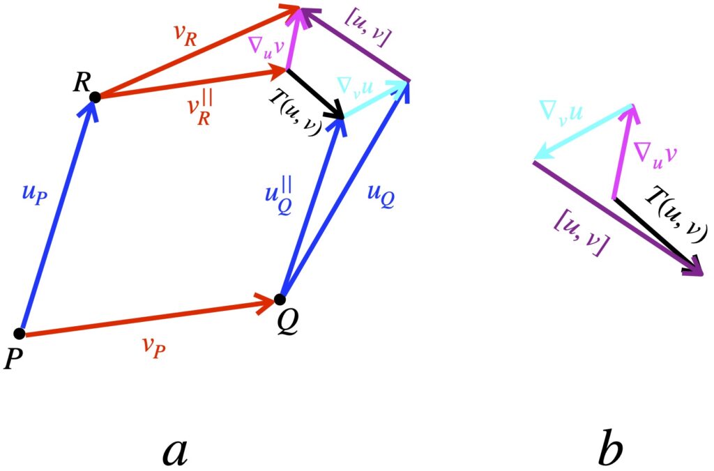
Figure 1a represents vectors that are part of vector fields (shown in blue) and  (shown in red). The vector
  represents the vector
  which has been parallel transported from point P to point Q. Similarly, the vector
  represents the vector
  which has been parallel transported from point P to point R. The difference between them is the torsion tensor
  .
.
In figure 1a,  represents the vector which has been Lie transported from P to Q. And
  represents the vector
  after it’s been Lie transported from P to R. The difference between these 2 vectors, shown in purple, is the Lie bracket
 ![\displaystyle \bigl[u,v\bigr]](https://www.samartigliere.com/wp-content/ql-cache/quicklatex.com-824f7a83dc9c6ab1b96627a4d35d4511_l3.png "Rendered by QuickLaTeX.com")
In the last 2 paragraphs and moving forward in this section, I’ve dropped the arrow above the letter notation since the context makes it clear that we’re dealing with vectors.
Figure 1b is a visual depiction of eq. (1). We start with the magenta vector labeled which represents the difference between the parallel transported vector and , a quantity given by the covariant derivative (as suggested by the label). We subtract from that the difference between and which, again, is the covariant derivative (represented by the cyan vector.) Next we subtract the Lie bracket (represented by the purple vector.) The result is the torsion tensor , shown in black. The torsion tensor is an operator that takes in 2 vectors and yields as its product a vector representing the difference between the 2 vectors parallel transported along each other.
If we set the torsion tensor to zero, that means the separation between the parallel transported vectors is zero which means we get a closed 4-sided shape, as shown in figure 2.
Image
Mathematically:
![\displaystyle T(u,v) = \nabla_{\vec{u}} \vec{v} -\nabla_{\vec{v}} \vec{u} - \bigl[\vec{u}, \vec{v}\bigr] = 0](https://www.samartigliere.com/wp-content/ql-cache/quicklatex.com-b424dfe2833a3af60ed2e44857e9ac82_l3.png "Rendered by QuickLaTeX.com")
![\displaystyle =\nabla_{\vec{u}} \vec{v} -\nabla_{\vec{v}} \vec{u} = \bigl[\vec{u}, \vec{v}\bigr] \quad \text{(2)}](https://www.samartigliere.com/wp-content/ql-cache/quicklatex.com-1db20c1fd23b97a7fddefa1a9f646489_l3.png "Rendered by QuickLaTeX.com")
When the above condition holds for all vector fields, we say the the connection is “torsion free.” It’s important to note, before going forward, that when we talk about torsion, we’re talking about the nature of the connection coefficients (e.g. Christoffel symbols.) It does not depend on the vector fields.
Now let’s find the components of the torsion tensor.
![\begin{align*} T(u,v) &= \nabla_{\vec{u}} \vec{v} -\nabla_{\vec{v}} \vec{u} - \bigl[\vec{u}, \vec{v}\bigr] \\ \\ &= \nabla_{\vec{u}} \vec{v} -\nabla_{\vec{v}} \vec{u} -\Bigl( \vec{u}(\vec{v}) - \vec{v}(\vec{u}) \Bigr) \\ \\ &=u^i \bigl( \partial _i v^k + v^j \Gamma^{k}_{ij} \bigr) \partial_k - v^i \bigl( \partial _i u^k + u^j \Gamma^{k}_{ij} \bigr) \partial_k \\ &\quad - \biggl[ \Bigl[ u^i \partial_i \bigl( v^j \partial_j \bigr) \Bigr] - \Bigl[ v^i \partial_i \bigl( u^j \partial_j \bigr) \Bigr] \biggr] \\ \\ &= u^i \bigl( \partial _i v^k + v^j \Gamma^{k}_{ij} \bigr) \partial_k - v^i \bigl( \partial _i u^k + u^j \Gamma^{k}_{ij} \bigr) \partial_k \\ &\quad - \biggl[ \Bigl[ u^i (\partial_i v^j)\partial_j + \cancel{u^iv^j(\partial_i\partial_j)} \Bigr] - \Bigl[ v^i (\partial_i u^j)\partial_j + \cancel{v^i u^j(\partial_i\partial_j)} \Bigr] \biggr]\\ \\ &= \bigl(u^i \partial _i v^k \partial_k + u^i v^j \Gamma^{k}_{ij} \partial_k \bigr) - \bigl( v^i \partial _i u^k \partial_k + v^i u^j \Gamma^{k}_{ij} \partial_k \bigr) \\ &\quad - \biggl[ u^i (\partial_i v^j)\partial_j - v^i (\partial_i u^j)\partial_j \biggr] \\ \\ &= \bigl( \cancel{u^i \partial _i v^k \partial_k} + u^i v^j \Gamma^{k}_{ij} \partial_k \bigr) - \bigl( \bcancel{v^i \partial _i u^k \partial_k} + v^i u^j \Gamma^{k}_{ij} \partial_k \bigr) \\ &\quad - \cancel{\biggl[ u^i (\partial_i v^k)\partial_k} - \bcancel{v^i (\partial_i u^k)\partial_k} \biggr] \\ \\ &= u^i v^j \Gamma^{k}_{ij} \partial_k - v^i u^j \Gamma^{k}_{ij} \partial_k \\ \\ &= u^i v^j \Gamma^{k}_{ij} \partial_k - v^j u^i \Gamma^{k}_{ji} \partial_k \\ \\ &= u^i v^j \Bigl( \Gamma^{k}_{ij} - \Gamma^{k}_{ji} \bigr) \partial_k \quad \text{(3)} \end{align*}](https://www.samartigliere.com/wp-content/ql-cache/quicklatex.com-ed5148b476a5940f6da6273ef9a31602_l3.png "Rendered by QuickLaTeX.com")
The term in parentheses are the components of the torsion tensor:
![\[ T^k_{ij} = \Gamma^{k}{ij} - \Gamma^{k}{ji} \quad \text{(4)} \]](https://www.samartigliere.com/wp-content/ql-cache/quicklatex.com-ccff3d0f41d459cba0aa35ae3c3c811a_l3.png "Rendered by QuickLaTeX.com")
When the torsion tensor is zero,  . Thus, the lower indices of the Christoffel symbols can be freely interchanged.
Eq. (4) also proves what we stated previously: namely, that the torsion tensor depends only on the connection coefficients, not on the coordinates.
II.F Geodesics
We’ve noted previously that, in an accelerated reference frame, and thus, in a gravitational field, light is predicted to follow a curved course. In fact, all objects tend to move along a path that’s as straight as possible (if not influenced by a non gravitational force), but in curved spacetime (like in a gravitational field), that path may be curved. Such motion is the general relativity version of Newton’s first law. Indeed, the natural state of motion of objects is said to be free fall, like that of the observer in the elevator plummeting toward earth, described in the introduction section.
We can formalize this mathematically in 2 ways:
II.F.1 Method 1
Since geodesic motion is the motion of free fall, and an observer in free fall experiences no acceleration, any mathematical description of such motion must include the fact that acceleration is zero. Accordingly, we need to start by coming up with a tensor expression for acceleration.
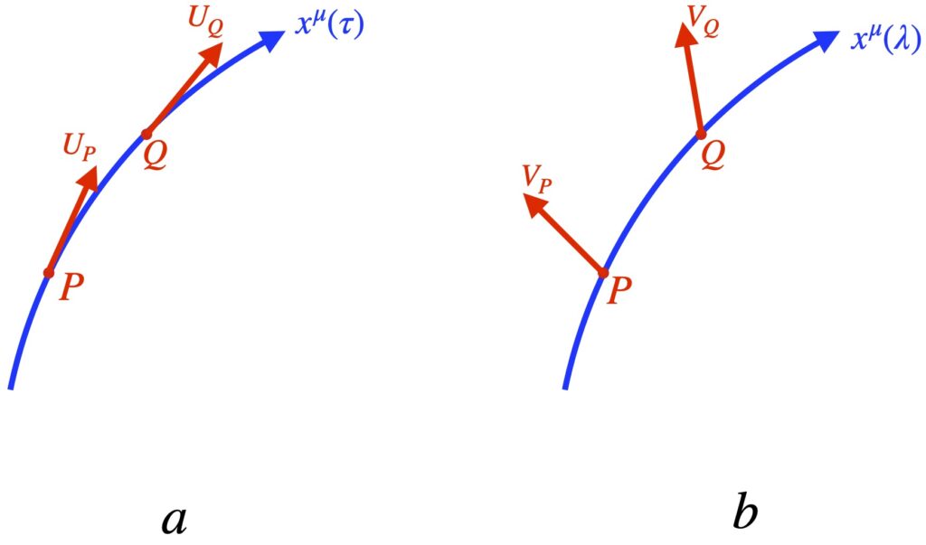
Referring to figure 2.5.1a, we can write a tensorial expression for acceleration as follows:

where  and
and  are velocity vectors on a worldline
  is geodesic parameterized by
  . Of course, velocity vectors are tangent vectors, and like all vectors, can be thought of as a derivative operator, in this case
  .
.  represents the vector parallel transported to point P so that a meaningful covariant derivative can be taken.
We’ve seen previously how to, in general, take a covariant derivative. Referring to figure 2.5.1b, we take and parallel transport it from point Q to point P on a worldline parameterized by , then us the following equation:

The components of the covariant derivative  , then, are :

where


Making the analogies  and
and  , we come up with the following tensor equation for the components of the acceleration:


Now,  . Therefore:


Since when traveling along a geodesic, there is no acceleration, we set eq. (2.5.6) to zero. We get:
![\[ \displaystyle \frac{\partial^2 x^{\mu}}{\partial \tau^2} + \Gamma^{\mu}_{\alpha \beta} \frac{\partial x^{\alpha}}{\partial \tau} \frac{\partial x^{\beta}}{\partial \tau} = 0 \quad \text{(2.5.7)} \]](https://www.samartigliere.com/wp-content/ql-cache/quicklatex.com-9dbcd3f8be9e78602e2649a95c219dd1_l3.png "Rendered by QuickLaTeX.com")
Eq. (2.5.7) is called the geodesic equation. This equation, in this form, applies to a timelike geodesic. If we were dealing with a spacelike geodesic, we’d replace with  . Lightlike geodesics are a little trickier. To write a valid geodesic equation for a lightlike geodesic, we’d use 4-momentum instead of 4-velocity in our equation as well as a parameter where
  , being mass. We take the limits
  and with
  remaining constant. For a more detailed explanation of the geodesic equation for lightlike geodesics, I refer you to
II.F.2 Method 2
This derivation is taken from Physics Unsimplified.
This second method of deriving the geodesic equation borrows the principle of stationary action from Lagrangian mechanics.
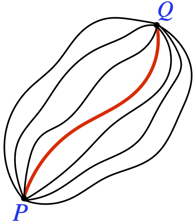
We imagine 2 points in spacetime, P and Q. There are an infinite number of possible paths, parameterized by some variable (say – proper time), that the particle could take in moving from P to Q. The path that the particle actually takes is the one that extremalizes the distance between P and Q,  . More information on this process and Lagrangian mechanics, in general, can be found here. We can apply this technique to arrive at the geodesic equation.
Figure 2.5.2 shows several worldlines – parameterized by – that a particle could follow between the points P and Q. The red worldline is the actual path taken by the particle (although we don’t know that before we start). The worldlines in the diagram are meant to be timelike but some, from the way they’re drawn, appear spacelike. Please excuse the deficiencies in my artwork. At any rate, we want to find the path that minimizes or maximizes the proper time it takes to traverse the path. We know that:

The worldlines are given by  . The velocity vectors (which are the tangent vectors) are given by
Now


Placing the results of eq. (2.5.10) into eq. (2.5.8), we get:

Next, we want to examine all of the possible paths by varying slightly, add up all the changes and see what the effect is on . The path that results in a minimum or maximum of – and the equation that describes that path – is the one that’s “picked out” by the process. It’s known that finding the minimum or maximum value of a function occurs when the first derivative is zero. Likewise, the extremal value of can be found when  . So the equation we need to solve is:

Differentiating using the product rule, we have:

![- \partial_{\alpha} g_{\mu \nu} \delta x^{\alpha} \dot{x}^{\mu} \dot{x}^{\nu} \Bigr) \biggr] \quad \text{(2.5.13)}](https://www.samartigliere.com/wp-content/ql-cache/quicklatex.com-baa14246051c99e32045a467fe58bed1_l3.png "Rendered by QuickLaTeX.com")
But 
Using this relationship in eq. (2.5.13), we get:
![\displaystyle \delta \tau = \int_P^Q d\lambda \biggl[ \frac{1}{\cancel{2} \sqrt{-g_{\mu \nu} \dot{x}^{\mu} \dot{x}^{\nu}}} \Bigl( -\cancel{2} g_{\mu \nu} \delta \dot{x}^{\mu} \dot{x}^{\nu} - \partial_{\alpha} g_{\mu \nu} \delta x^{\alpha} \dot{x}^{\mu} \dot{x}^{\nu} \Bigr) \biggr] \quad \text{(2.5.15)}](https://www.samartigliere.com/wp-content/ql-cache/quicklatex.com-6d3400a7bcc5e75da031bef561c19115_l3.png "Rendered by QuickLaTeX.com")
Next, we integrate by parts. The following is a brief recap of how integration by parts works.
![\displaystyle \int \dfrac{d}{dx}\left[ F(x)G(x)\right]dx = \int_a^b F\left( x\right) \dfrac{dG}{dx}dx+\int G\left( x\right) \dfrac{dF}{dx}dx](https://www.samartigliere.com/wp-content/ql-cache/quicklatex.com-36e1cfe78fe7bbf09e942e09dfb614a3_l3.png "Rendered by QuickLaTeX.com")
![\displaystyle \int \dfrac{d}{dx}\left[ F(x)G(x)\right] dx-\int G\left( x\right) \dfrac{dF}{dx}dx=\int F\left( x\right) \dfrac{dG}{dx}dx](https://www.samartigliere.com/wp-content/ql-cache/quicklatex.com-6de153ddd87247e85260790540183f3e_l3.png "Rendered by QuickLaTeX.com")

In our case:


Applying integration by parts to the term  , we obtain:
![\displaystyle \delta \tau = -\displaystyle \frac{g_{\mu \nu}\dot{x}^{\nu}}{\sqrt{-g_{\mu \nu} \dot{x}^{\mu} \dot{x}^{\nu}}}} \eval{\delta x^{\mu}}_P^Q + \int_P^Q d\lambda \biggl[ \frac{d}{d\lambda}\left( \frac{g_{\mu \nu}\dot{x}^{\nu}}{\sqrt{-g_{\mu \nu} \dot{x}^{\mu} \dot{x}^{\nu}}}} \right) \delta x^{\mu} - \frac{\partial_{\alpha} g_{\mu \nu} \dot{x}^{\mu} \dot{x}^{\nu}}{2\sqrt{-g_{\mu \nu} \dot{x}^{\mu} \dot{x}^{\nu}}}} \delta x^{\alpha} \biggr] \quad \text{(2.5.16)}](https://www.samartigliere.com/wp-content/ql-cache/quicklatex.com-bcc9b5bfbdc88cc47685986860f243d9_l3.png "Rendered by QuickLaTeX.com")
Points P and Q are fixed; they don’t vary. Thus,  . Therefore the term
  . This makes eq. (2.5.16):
![\displaystyle \delta \tau = \int_P^Q d\lambda \biggl[ \frac{d}{d\lambda}\left( \frac{g_{\mu \nu}\dot{x}^{\nu}}{\sqrt{-g_{\mu \nu} \dot{x}^{\mu} \dot{x}^{\nu}}}} \right) \delta x^{\mu} - \frac{\partial_{\alpha} g_{\mu \nu} \dot{x}^{\mu} \dot{x}^{\nu}}{2\sqrt{-g_{\mu \nu} \dot{x}^{\mu} \dot{x}^{\nu}}}} \delta x^{\alpha} \biggr] \quad \text{(2.5.17)}](https://www.samartigliere.com/wp-content/ql-cache/quicklatex.com-3a10c2527928c528dd308ccc89dff39f_l3.png "Rendered by QuickLaTeX.com")
We’d like to factor out the  terms but they have different indices. We can fix this by making the following dummy index changes in the righthand term: and
  . That gives us:
![\displaystyle \delta \tau = \int_P^Q d\lambda \biggl[ \frac{d}{d\lambda}\left( \frac{g_{\mu \nu}\dot{x}^{\nu}}{\sqrt{-g_{\mu \nu} \dot{x}^{\mu} \dot{x}^{\nu}}}} \right) - \frac{\partial_{\mu} g_{\alpha \beta} \dot{x}^{\alpha} \dot{x}^{\beta}}{2\sqrt{-g_{\mu \nu} \dot{x}^{\mu} \dot{x}^{\nu}}}} \delta x^{\mu} \biggr] \delta x^{\mu} \quad \text{(2.5.18)}](https://www.samartigliere.com/wp-content/ql-cache/quicklatex.com-d09356effd26281358eebd0bceb68197_l3.png "Rendered by QuickLaTeX.com")
We want to extremize the proper time so we set  . The only way this can happen is if the term in bracket is zero. That yields:

Eq. (2.5.19) is true for any arbitrary parameter lambda. Thus, it still holds if we set  . When we do this, the
  terms become
  where
where  represents the 4-velocity. But we know that the dot product of the 4-velocity is -1 (in units where c=1). Thus:

When we substitute this result into eq. (2.5.19), eq. (2.5.19) becomes:


Multiplying both sides of eq. (2.5.20) by  changes eq. (2.5.20) to:

We’d like to factor out a factor of  from the righthand term of eq. (2.5.21). To do this, we have to change the dummy index
  in the lefthand term in the parentheses. We have:

Because is symmetric in their indices, this means that  so we can replace the term
  with the expression
  . We get:


Eq. (2.5.23), of course, is the geodesic equation, which is what we were trying to derive.
Local Inertial Frame
I mentioned earlier that, even in curved spacetime, spacetime, over small regions, spacetime looks flat. And I said that I’d offer a proof later. Now, with some additional mathematical tools in our toolkit, I’m in a position to provide that proof.
The above statement – that in small regions, spacetime will look flat – can also be expressed in the following manner: For each tiny region in spacetime, coordinates can be chosen such that the observed metric is the Minkowski metric (i.e., spacetime appears flat). Such coordinates are called Fermi normal coordinates. Proof of this is tedious. However, for those interested, a proof of this can be found .
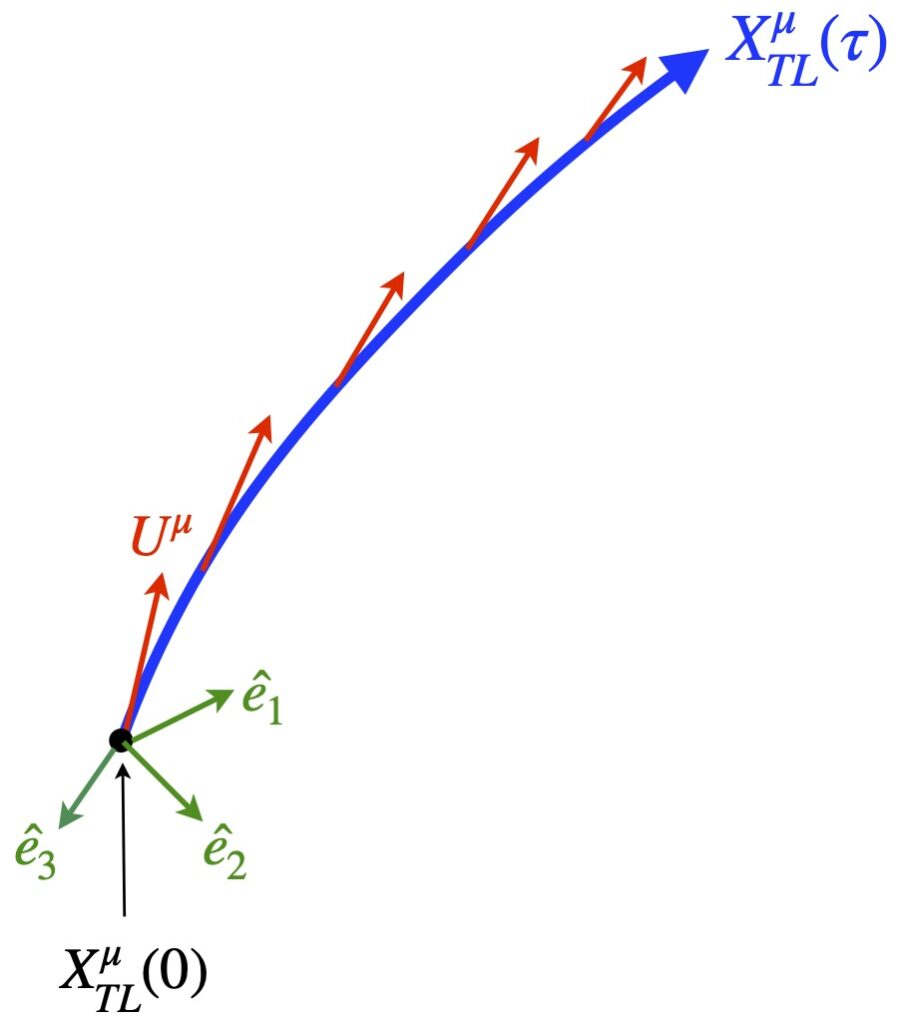
![\[X^{\mu}_{TL}(\tau)\quad \text{eq (1)} \]](https://www.samartigliere.com/wp-content/ql-cache/quicklatex.com-71e25b7f8883bfd11572798b1e9aa141_l3.png "Rendered by QuickLaTeX.com")
 are the 4 vector’s spacetime coordinates
 indicates that this is a time-like geodesic
 indicates that the displacement vector’s components are a function of proper time
 are the components of the 4-velocity along the worldline, which, of course, is tangent to and parallel transported along, the worldline.
 vectors are space-like unit vectors that form an orthonormal basis at the origin of the world line,
  , where
![\[ a^{\mu} = \frac{D \,U^{\mu}}{D \,\tau} = \frac{dX^{\alpha}}{d\tau}\frac{dU^{\mu}}{dX^{\alpha}} = U^{\alpha} \nabla_{\alpha} U^{\mu} = 0 \quad \text{eq (2)} \]](https://www.samartigliere.com/wp-content/ql-cache/quicklatex.com-daef768f59d9cc588bb45f17fb1d3425_l3.png "Rendered by QuickLaTeX.com")
 (i.e., the inner product of the 4-velocity is -1 when we set
  (i.e., the space-like basis vectors are orthogonal)
 (i.e., the space-like basis vectors are orthogonal to the 4-velocity vector which is tangent to the worldline)
 , along the worldline defined by
  , then the covariant derivative is zero:
![\[ U^{\alpha}\nabla_{\alpha}e^{\mu}_a = 0 \quad \text{eq (6)} \]](https://www.samartigliere.com/wp-content/ql-cache/quicklatex.com-4420351cee4dc510a9cdb87e34db3b09_l3.png "Rendered by QuickLaTeX.com")
 and
and  is orthonormal at point O, at the origin. What we need to do is show that they are orthonormal at all points along the worldline. To do this, we need to demonstrate that the the derivative of
  with respect to time is zero (i.e., does not change) everywhere along the worldline:
 , indicates that the spacelike basis vectors,
  , are orthogonal. By showing that the derivative with respect to proper time of this expression equals zero, we show that this orthogonal configuration does not change as we move along our timeline worldline:
 basis vectors at every point along the worldline. From these facts, we can extract a couple of equations that we’ll need later:
![\[ U^{\alpha}\nabla_{\alpha}U^{\mu} = \ddot{x}^{\mu}_{TL} + \eval {\Gamma^{\mu}_{\alpha \beta}}_{TL} \dot{x}^{\alpha}_{TL}\,\dot{x}^{\beta}_{TL} = 0 \quad \text{eq (9)} \]](https://www.samartigliere.com/wp-content/ql-cache/quicklatex.com-316a2b23c3bed511c069632f7782eaf1_l3.png "Rendered by QuickLaTeX.com")

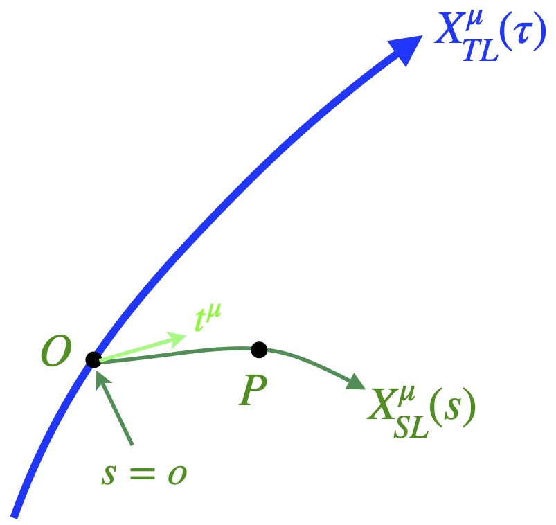
 where the subscript
  indicates that it is spacelike, and again,
  , is tangent to this spacelike geodesic and point P is a point along that geodesic:
![\[ t=\frac{\partial}{\partial s} \,\, \Rightarrow \,\, t^{\mu} = \frac{\partial X^{\mu}_{SL}(s)}{\partial s} \quad \text{eq (11)} \]](https://www.samartigliere.com/wp-content/ql-cache/quicklatex.com-9ca367918a6a04ae31d9dc8087f7df0f_l3.png "Rendered by QuickLaTeX.com")
 basis:
![\[ t^{\mu} = t^a\hat{e}^{\mu}_a \quad \text{eq (12)} \]](https://www.samartigliere.com/wp-content/ql-cache/quicklatex.com-21c2fb269ca4c12b94b244101476b55f_l3.png "Rendered by QuickLaTeX.com")
![\[ \eval{X^{\mu}}_P = X^{\mu}_{SL}(0) + \dot{x}_{SL}(0)s + \frac12\ddot{X}_{SL}(0)s^2 + \dots \quad \text{eq (13)} \]](https://www.samartigliere.com/wp-content/ql-cache/quicklatex.com-7efd1b99337080b8152b0bf20f8a584d_l3.png "Rendered by QuickLaTeX.com")
 represents
  , the coordinates at point O,
  .
. represents
  , the spacelike tangent vector at point O,
  .
. represents higher order terms (which are negligible).

 depends on point O but
  does not.
 ) from our old coordinates (
 ). These new coordinates are called Fermi normal coordinates and are given by:
 ![\[ X^{\mu}(\tau,\bar{x}^a) = X^{\mu}_{SL}(\tau) + \bar{x}^a e^{\mu}_a - \frac12 \eval {\Gamma^{\mu}_{\alpha \beta}}_{X_{TL}(\tau)} \bar{x}^a \, \bar{x}^b \, e^{\alpha}_a(\tau) e^{\alpha}_b(\tau) + \dots \,\, \text{eq (16)} \]](https://www.samartigliere.com/wp-content/ql-cache/quicklatex.com-131729149cb205f08037e8fe3dbe9fa2_l3.png "Rendered by QuickLaTeX.com")

 is the direction of the spacelike coordinate and

 , we need to compute
  and
and  from eq (16):
![\[ X^{\mu}(\tau,\bar{x}^a) = X^{\mu}_{SL}(\tau) + \bar{x}^a e^{\mu}_a - \frac12 \eval {\Gamma^{\mu}_{\alpha \beta}}_{X_{TL}(\tau)} \underbrace{\bar{x}^a \, \bar{x}^b}_{\bar{x}^2} \, e^{\alpha}_a(\tau) e^{\alpha}_b(\tau) + \dots \,\, \text{eq (16)} \]](https://www.samartigliere.com/wp-content/ql-cache/quicklatex.com-dde8619b0b4e1ca67eaf7ba1503caf7e_l3.png "Rendered by QuickLaTeX.com")
 term is quadratic in
  . Thus, this and higher order terms are negligible. When we take the derivative with respect to
 basis vectors so we can use eq (10) that we derived previously:
 into eq (18), we obtain:
![\[ \boxed{\frac{\partial X^{\mu}}{\partial \tau} = U^{\mu} -\Gamma^{\mu}_{\alpha \beta} U^{\alpha} \bar{x}^a e^{\beta}_{a} + \dots \quad \text{eq (20)}} \]](https://www.samartigliere.com/wp-content/ql-cache/quicklatex.com-c85df88d4ffe7b987b4c1cff73fea218_l3.png "Rendered by QuickLaTeX.com")
 . For convenience, I’ll reproduce the equation for Fermi normal coordinates, eq (16), here:
![\[ X^{\mu}(\tau,\bar{x}^a) = X^{\mu}_{SL}(\tau) + \bar{x}^a e^{\mu}_a - \frac12 \eval {\Gamma^{\mu}_{\alpha \beta}}_{X_{TL}(\tau)} \bar{x}^a \, \bar{x}^b \, e^{\alpha}_a(\tau) e^{\alpha}_b(\tau) + \dots \]](https://www.samartigliere.com/wp-content/ql-cache/quicklatex.com-fc29c4802fd77b4c90d4191704206164_l3.png "Rendered by QuickLaTeX.com")

![\[ \boxed{\frac{\partial X^{\mu}}{\partial \bar{x}^c} = e^{\mu}_c - \Gamma^{\mu}_{\alpha \beta} \bar{x}^b e^{\beta}_b e^{\alpha}_c + \dots \quad \text{eq (22)}} \]](https://www.samartigliere.com/wp-content/ql-cache/quicklatex.com-bace4ea797eca3b99581b71746e3d083_l3.png "Rendered by QuickLaTeX.com")
 =
=  + tiny corrections


![+ \partial_{\alpha} g_{\mu \nu} \bar{x}^d e^{\alpha}_d U^{\mu} - \partial_{\alpha} g_{\mu \nu} \bar{x}^d e^{\alpha}_d \Gamma^{\mu}_{\alpha \beta} U^{\alpha} \bar{x}^a e^{\beta}_{a}] \cdot](https://www.samartigliere.com/wp-content/ql-cache/quicklatex.com-070358b0d63619c7c281b8f3b7613be1_l3.png "Rendered by QuickLaTeX.com")
![[ U^{\nu} -\Gamma^{\nu}_{\sigma \rho} U^{\rho} \bar{x}^b e^{\alpha}_{b} ]](https://www.samartigliere.com/wp-content/ql-cache/quicklatex.com-fb88877b995191357f6c90d97afd8709_l3.png "Rendered by QuickLaTeX.com")


 =-c^2 (when the mostly-pluses form of the metic is employed). Setting
  =
=  + tiny corrections


![- \partial_{\alpha}g_{\mu \nu} \bar{x}^d e^{\alpha}_d \Gamma^{\mu}_{\alpha \beta} U^{\alpha} \bar{x}^a e^{\beta}_{a}]\cdot [e^{\mu}_c - \frac12\Gamma^{\mu}_{\alpha \beta} \bar{x}^b e^{\beta}_b e^{\alpha}_c]](https://www.samartigliere.com/wp-content/ql-cache/quicklatex.com-39bd92c199943b966152b677129aa01f_l3.png "Rendered by QuickLaTeX.com")
![\approx \underbrace{\cancel{g_{\mu \nu}U^{\mu}e^{\mu}_c}}_{0} - g_{\mu \nu}U^{\mu}\frac12\Gamma^{\mu}_{\alpha \beta} \bar{x}^b e^{\beta}_b e^{\alpha}_c] -g_{\mu \nu} \Gamma^{\mu}_{\alpha \beta} U^{\alpha} \bar{x}^b e^{\beta}_b e^{\nu}_a](https://www.samartigliere.com/wp-content/ql-cache/quicklatex.com-4ba5c908a6f9c4070c1514d48e02d260_l3.png "Rendered by QuickLaTeX.com")


 . We’re dealing with the case where
  . Therefore,
  2 are negligible and can be ignored.
![\bar{g}_{\tau a} \approx - g_{\mu \nu}U^{\mu}\Gamma^{\mu}_{\alpha \beta} \bar{x}^b e^{\beta}_b e^{\alpha}_c]](https://www.samartigliere.com/wp-content/ql-cache/quicklatex.com-96b53edf81ca465ddf4e334ae07acac5_l3.png "Rendered by QuickLaTeX.com")


![\approx - \frac12 g_{\mu \nu}U^{\mu} g^{\nu \gamma} (\partial_{\sigma}g_{\rho \gamma} + \partial_{\rho}g_{\sigma \gamma} + \partial_{\alpha}g_{\sigma \rho}) \bar{x}^b e^{\beta}_b e^{\alpha}_c]](https://www.samartigliere.com/wp-content/ql-cache/quicklatex.com-b5c7b21c4560e2295d68d00c3b7170db_l3.png "Rendered by QuickLaTeX.com")

![\approx - \frac12 \underbrace{g_{\mu \nu}g^{\nu \gamma}}_{\delta^{\gamma}_{\mu}} U^{\mu} (\partial_{\sigma}g_{\rho \gamma} + \partial_{\rho}g_{\sigma \gamma} + \partial_{\alpha}g_{\sigma \rho}) \bar{x}^b e^{\beta}_b e^{\alpha}_c]](https://www.samartigliere.com/wp-content/ql-cache/quicklatex.com-9bc3848dde67370c4a83e35b979a42ab_l3.png "Rendered by QuickLaTeX.com")

![\approx - \frac12 U^{\mu} (\partial_{\sigma}g_{\rho \mu} + \partial_{\rho}g_{\sigma \mu} + \partial_{\mu} g_{\sigma \rho}) \bar{x}^b e^{\beta}_b e^{\alpha}_c]](https://www.samartigliere.com/wp-content/ql-cache/quicklatex.com-cec4a0fd43067ebe0ef4dc6e49ae52dd_l3.png "Rendered by QuickLaTeX.com")


 =
=  + tiny corrections


 and
and  are the same. Since they have opposite signs, they cancel. Likewise, the last term on the righthand side is quadratic in
  and is, therefore, negligible. That leaves us with:

 + tiny corrections
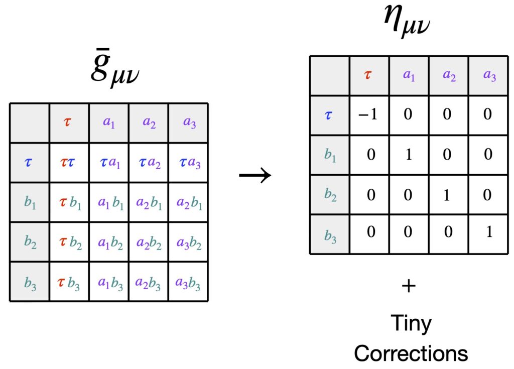
 If you look at the solutions for the individual components, you’ll see that the “tiny corrections” described to in eq (23) (and the equations before it) are due to terms that are quadratic and higher power terms. Specifically, they refer to a spacelike coordinate
  which, as described above, points outward from our timeline geodesic, in the direction of
  – at a point on the geodesic – becomes equal to the Minkowski metric
  .
.

 . On the timelike geodesic,
  and so
  .
.![\[\overline{\nabla}_{\alpha}\overline{T}^{\dots}_{\dots} = \overline{\partial}_{\alpha}\overline{T}^{\dots}_{\dots}\]](https://www.samartigliere.com/wp-content/ql-cache/quicklatex.com-7d13d8f507746a740651e31938fa1279_l3.png "Rendered by QuickLaTeX.com")
Riemann Curvature Tensor
With the concepts of the covariant derivative and parallel transport in hand, we’re now ready to find a method for determining whether a space is flat or curved.
Derivation
The derivation that follows is taken from Robert Davies, “Riemann Curvature Tensor” which is part of his Tensor Calculus series on YouTube.
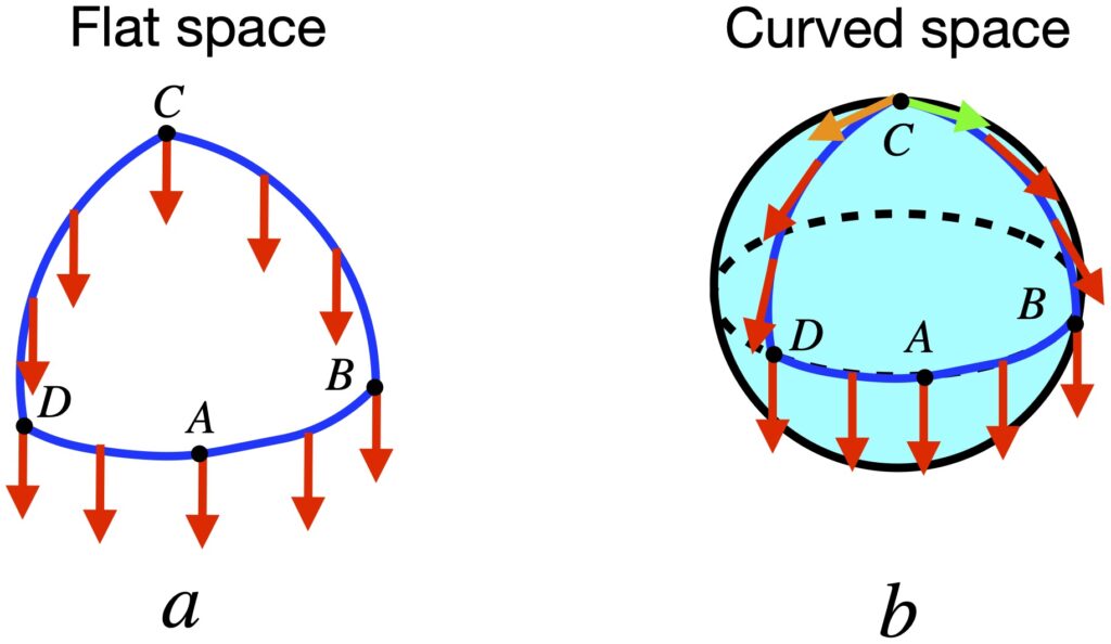
We can see, from figure 2.6.1a, that when we parallel transport a vector from point A to B to C, it will remain unchanged as compared with the same vector parallel transported from A to D to C. However, in curved space like the surface of a sphere (see figure 2.6.2), when we parallel transport a vector from A to B to C, the vector that we end up with at C will differ from the resultant vector after parallel transporting the same vector from A to D to C. To determine whether a space is flat or curved, we’ll apply this same basic idea of parallel transport of a vector in different directions around a closed loop, but will examine this process on a loop of infinitesimal length.
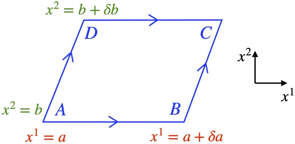
Specifically, as shown in figure 2.6.2, we’ll take a vector, , and, like in figure 2.6.1 parallel transport it to point C along 2 paths – A to B to C and A to D to C. For each path, we’ll write equations describing these motions with a goal of arriving at a mathematical expression that characterizes the curvature of the space in which we’re working.
Before we get into the derivation proper, we know that we can consider derivatives as operators that bring about changes in functions. Allowing for minor abuses in notation, we can write:

Similarly, we can think of the covariant derivative as an operator that brings about a change in a vector as it’s parallel transported along a worldline. For example:

where we sum up all the little changes brought about by our operator (the covariant derivative), in each little interval,  , take the limit as x goes to zero and add it to the initial vector to get the total change.
We also know that, since the covariant derivative of a vector that’s parallel transported is zero, we can use equations like the following:

which implies:

Given these tools, let’s begin with parallel transport of vector from A to B along the  . We have:

Note that in eq. (2.6.5), and subsequently in this discussion, we’ve moved  to the left side of the equation.
The equations for parallel transport of  from B to C are:
![\[ \frac{\partial v^{\alpha}}{\partial x^{2}} & =-v^{\mu} \Gamma_{\mu 2}^{\alpha} \quad \text{(2.6.6)} \]](https://www.samartigliere.com/wp-content/ql-cache/quicklatex.com-cc7c536478cdd9f8ed92a0367c2d52cd_l3.png "Rendered by QuickLaTeX.com")
and

The net change for Path 1 (i.e., the path from A to B to C) is:

Next, we turn our attention to Path 2, the path from A to D to C. We’ll begin with parallel transport from A to D. We have:

The equations for parallel transport from D to C are:

For the entirety of Path 2, the equations are:

The difference between the vectors transported along Path 1 and Path 2, when they get to C, is given by:

We rearrange terms such that  terms and
  terms are together:

Notice that the integrands in the integrals  (which represents transported from A to D) and
  (which represents transported from B to C), are the same. These vectors are parallel but separated by . What we’d like to do is parallel transport the
  vector to the
  vector so we can compare them directly. This will give us the
  component of the
  . To do this, we take the Taylor series expansion of the vector at D in the direction. Or, the way I like to think about is: take the vector at D and parallel transport it to the resultant BC vector at C by taking the derivative of the vector at D with respect to , then multiply it by
  – the infinitesimal displacement to C – similar to what we did in parallel transporting our other vectors.
Likewise, the vectors resulting from parallel transport from D to C and A to B are parallel. Thus, we’ll compare them in the manner described above for the A to D and B to C parallel transported vectors to get the component of . The results are:
![\begin{align*} \delta v^{\alpha}& =-\int_{A D}\left(v^{\mu} \Gamma_{\mu 2}^{\alpha}+\delta a \frac{\partial}{\partial x^{1}}\left(v^{\mu} \Gamma_{\mu 2}^{\alpha}\right) \ldots\right) d x^{2}+\int_{B C} v^{\mu} \Gamma_{\mu 2}^{\alpha} d x^{2} \\ &\quad-\int_{D C} v^{\mu} \Gamma_{\mu 1}^{\alpha} d x^{1}+\int_{A B}\left(v^{\mu} \Gamma_{\mu 1}^{\alpha}+\delta b \frac{\partial}{\partial x^{2}}\left(v^{\mu} \Gamma_{\mu 1}^{\alpha}\right) \ldots\right) d x^{1} \\ \\ &= \int_{b}^{b +\delta b} \Biggl[-v^{\mu} \Gamma_{\mu 2}^{\alpha}-\left(\delta a \frac{\partial}{\partial x^{1}}\left(v^{\mu} \Gamma_{\mu 2}^{\alpha}\right) \ldots\right) +v^{\mu} \Gamma_{\mu 2}^{\alpha}\Biggr] d x^{2} \\ &\quad\int_a^{a+\delta a} \Biggl[-v^{\mu} \Gamma_{\mu 1}^{\alpha} +v^{\mu} \Gamma_{\mu 1}^{\alpha}+\left(\delta b \frac{\partial}{\partial x^{2}}\left(v^{\mu} \Gamma_{\mu 1}^{\alpha}\right) \ldots\right)\Biggr] d x^{1} \quad \text{(2.6.14)} \end{align*}](https://www.samartigliere.com/wp-content/ql-cache/quicklatex.com-13b2f67aa9909cec1d07c82f745bdd08_l3.png "Rendered by QuickLaTeX.com")
After cancelling the  terms of opposite sign in eq. (2.6.14), we’re left with:
![\[ \int_{b}^{b +\delta b} -\delta a \frac{\partial}{\partial x^{1}}\Bigl(v^{\mu} \Gamma_{\mu 2}^{\alpha}\Bigr)\,\,dx^2 + \int_a^{a+\delta a} \delta b \frac{\partial}{\partial x^{2}}\Bigl(v^{\mu} \Gamma_{\mu 1}^{\alpha}\Bigr)\,\, dx^1 \quad \text{(2.6.15)} \]](https://www.samartigliere.com/wp-content/ql-cache/quicklatex.com-e107ac0a6ebe440e8b984828f6482a7c_l3.png "Rendered by QuickLaTeX.com")
This next step is where I become confused. In the video from Robert Davie and other sources that present this derivation (e.g., Scott Hughes, General Relativity, at 1h 05min of Lecture 10, MIT Opencourseware; Bernard Schutz, A First Course in General Relativity, p. 159), it’s said that, because we’re working with infinitesimal distances, the integrals in eq. (2.6.15) become just the area of the loop, . Thus, we can pull out the
  ,
,  terms and dispense with the integral to get:
![\[ \delta a \delta b \Bigl[ -\frac{\partial}{\partial x^{1}}\Bigl(v^{\mu} \Gamma_{\mu 2}^{\alpha}\Bigr) + \frac{\partial}{\partial x^{2}}\Bigl(v^{\mu} \Gamma_{\mu 1}^{\alpha}\Bigr) \Bigr] \quad \text{(2.6.16)} \]](https://www.samartigliere.com/wp-content/ql-cache/quicklatex.com-10206c8ba1af5ec5e8a717add9f3a37a_l3.png "Rendered by QuickLaTeX.com")
To see how I reconcile this, click .
 : when we take the integral
  , we get
  , leaving us with
 ![\delta a \delta b \Bigl[ -\frac{\partial}{\partial x^{1}}\Bigl(v^{\mu} \Gamma_{\mu 2}^{\alpha}\Bigr) \Bigr]](https://www.samartigliere.com/wp-content/ql-cache/quicklatex.com-3138ef3ae37e013662f8dcd11f867b28_l3.png "Rendered by QuickLaTeX.com") .
. : when we take the integral
  , we get
  , leaving us with
 ![\delta a \delta b \Bigl[ \frac{\partial}{\partial x^{2}}\Bigl(v^{\mu} \Gamma_{\mu 1}^{\alpha}\Bigr) \Bigr]](https://www.samartigliere.com/wp-content/ql-cache/quicklatex.com-11876a0bafd6483c24d8ef5df04615ee_l3.png "Rendered by QuickLaTeX.com") .
.![\[ \delta a \delta b \Bigl[ -\frac{\partial}{\partial x^{1}}\Bigl(v^{\mu} \Gamma_{\mu 2}^{\alpha}\Bigr) + \frac{\partial}{\partial x^{2}}\Bigl(v^{\mu} \Gamma_{\mu 1}^{\alpha}\Bigr) \Bigr] \]](https://www.samartigliere.com/wp-content/ql-cache/quicklatex.com-cd7b28aeb1314d03877cffc573aa1d0c_l3.png "Rendered by QuickLaTeX.com")
At this point, we expand out the expression in the brackets in eq. (2.6.16) using the product rule, swap some dummy indices and where appropriate, make the following substitution for partial derivatives:  . This leads to:
![\begin{align*} \delta v^\alpha & \approx \delta a \delta b\left[-\frac{\partial}{\partial x^1}\left(v^\mu \Gamma_{\mu 2}^\alpha\right)+\frac{\partial}{\partial x^2}\left(v^\mu \Gamma_{\mu 1}^\alpha\right)\right] \\ & =\delta a \delta b\left[\frac{\partial v^\mu}{\partial x^2} \Gamma_{\mu 1}^\alpha+\frac{\partial \Gamma_{\mu 1}^\alpha}{\partial x^2} v^\mu-\frac{\partial v^\mu}{\partial x^1} \Gamma_{\mu 2}^\alpha-\frac{\partial \Gamma_{\mu 2}^\alpha}{\partial x^1} v^\mu\right] \\ & =\delta a \delta b\left[-v^v \Gamma_{v 2}^\mu \Gamma_{\mu 1}^\alpha+\frac{\partial \Gamma_{\mu 1}^\alpha}{\partial x^2} v^\mu--v^v \Gamma_{v 1}^\mu \Gamma_{\mu 2}^\alpha-\frac{\partial \Gamma_{\mu 2}^\alpha}{\partial x^1} v^\mu\right] \\ & =\delta a \delta b\left[-v^\mu \Gamma_{\mu 2}^v \Gamma_{v 1}^\alpha+\frac{\partial \Gamma_{\mu 1}^\alpha}{\partial x^2} v^\mu--v^\mu \Gamma_{\mu 1}^v \Gamma_{v 2}^\alpha-\frac{\partial \Gamma_{\mu 2}^\alpha}{\partial x^1} v^\mu\right] \\ & =\delta a \delta b\left[\frac{\partial \Gamma_{\mu 1}^\alpha}{\partial x^2} v^\mu-\frac{\partial \Gamma_{\mu 2}^\alpha}{\partial x^1} v^\mu+\Gamma_{\mu 1}^v \Gamma_{v 2}^\alpha v^\mu-\Gamma_{\mu 2}^v \Gamma_{v 1}^\alpha v^\mu\right] \\ & =\delta a \delta b\left[\frac{\partial \Gamma_{\mu 1}^\alpha}{\partial x^2}-\frac{\partial \Gamma_{\mu 2}^\alpha}{\partial x^1}+\Gamma_{\mu 1}^v \Gamma_{v 2}^\alpha-\Gamma_{\mu 2}^v \Gamma_{v 1}^\alpha\right] v^{\mu} \quad \text{(2.6.17)} \end{align*}](https://www.samartigliere.com/wp-content/ql-cache/quicklatex.com-bfdcd170403d924dc1829d97ebaf0d9d_l3.png "Rendered by QuickLaTeX.com")
When we take the limit as and go to zero, we get the difference in the parallel transported vectors at point C:
![\[ \delta v^\alpha = \Bigl[ \frac{\partial \Gamma_{\mu 1}^\alpha}{\partial x^2}-\frac{\partial \Gamma_{\mu 2}^\alpha}{\partial x^1}+\Gamma_{\mu 1}^v \Gamma_{v 2}^\alpha-\Gamma_{\mu 2}^v \Gamma_{v 1}^\alpha\Bigr] v^{\mu} \quad \text{(2.6.18)}\]](https://www.samartigliere.com/wp-content/ql-cache/quicklatex.com-eb5e1d01fd07f806a923db0cc2418490_l3.png "Rendered by QuickLaTeX.com")
When  = 0, it means the space we’re working with is flat. If it’s nonzero, it means the space is curved. The operator that ultimately makes this differentiation is the expression in brackets in eq. (2.6.18):
![\[\delta v^{\alpha} = R^{\alpha}_{\mu21} = \frac{\partial \Gamma_{\mu 1}^\alpha}{\partial x^2}-\frac{\partial \Gamma_{\mu 2}^\alpha}{\partial x^1}+\Gamma_{\mu 1}^v \Gamma_{v 2}^\alpha-\Gamma_{\mu 2}^v \Gamma_{v 1}^\alpha \quad \text{(2.6.19)} \]](https://www.samartigliere.com/wp-content/ql-cache/quicklatex.com-3c9f5ab419591cba368ce8624d3d5bf5_l3.png "Rendered by QuickLaTeX.com")
We can make this more general by generalizing the coordinate lines and , replacing them with  and
and  :
:
![\[ R^{\alpha}_{\mu \gamma \beta} = \frac{\partial \Gamma_{\mu \beta}^\alpha}{\partial x^\gamma}-\frac{\partial \Gamma_{\mu \gamma}^\alpha}{\partial x^\beta}+\Gamma_{\mu \beta}^v \Gamma_{v \gamma}^\alpha-\Gamma_{\mu \gamma}^v \Gamma_{v \beta}^\alpha \quad \text{(2.6.20)} \]](https://www.samartigliere.com/wp-content/ql-cache/quicklatex.com-787a11123363c04841283a45babeee14_l3.png "Rendered by QuickLaTeX.com")
So we can think of the Riemann curvature tensor as an operator which takes 3 vectors as an inputs (2 infinitesimal displacement vectors and the vector it will parallel transport) and spits out the difference vector , which tells us whether a space is flat or curved.
Method 2
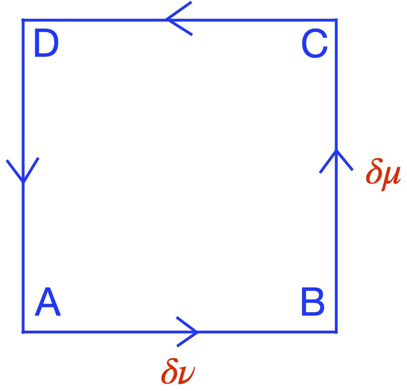
Another way to derive an expression for the Riemann curvature tensor is to make use of a mathematical object referred to as a commutator. Again, we consider parallel transport of a vector,  , around an infinitesimal square closed loop defined by 2 vectors,
  and
and  . The lengths of sides of this infinitesimal square are
  and
and  , respectively.
We start by parallel transporting from A to B. We know that the operator that brings about parallel transport is the covariant derivative. Thus, we can describe this movement from A to B mathematically as:
![\[ \nabla_{\nu}V^{\lambda} \delta \nu\quad \text{(2.6.21)} \]](https://www.samartigliere.com/wp-content/ql-cache/quicklatex.com-bf583be8f23d32f387ebdac940167fb1_l3.png "Rendered by QuickLaTeX.com")
We then parallel transport the resultant vector at B to point C via the covariant derivative in the direction as follows:
![\[ \nabla_{\mu} \delta \mu \bigl(\nabla_{\nu}V^{\lambda}\bigr) \delta \nu \quad \text{(2.6.22)}\]](https://www.samartigliere.com/wp-content/ql-cache/quicklatex.com-4c1c91daf0b398bc08949972db997228_l3.png "Rendered by QuickLaTeX.com")
Therefore, the expression describing the transport of from A to B to C is:
![\[ \nabla_{\mu} \nabla_{\nu}V^{\lambda} \delta \mu \delta \nu \quad \text{(2.6.23)}\]](https://www.samartigliere.com/wp-content/ql-cache/quicklatex.com-ff00eb1339d6d4b4fdb595cce3439441_l3.png "Rendered by QuickLaTeX.com")
Now, like in method 1 derivation described above, we want to parallel transport from A to D to C. Then we subtract the vector at C resulting from this path from vector resulting from transport along the A to B to C path. Again, if the result is zero (i.e., no difference), then we infer that the space is flat along this loop. If the result is nonzero (i.e., there is a difference) then we presume that the space is curved in the area of the loop. And if we take the limit as and go to zero, we can determine the flatness or curvature at the point C.
So, in parallel transporting from A to D, we move along the direction. Thus, we have:
![\[ \nabla_{\mu}V^{\lambda} \delta \mu\quad \text{(2.6.24)} \]](https://www.samartigliere.com/wp-content/ql-cache/quicklatex.com-210adbd1cd9f91181406d3dc5b2923e1_l3.png "Rendered by QuickLaTeX.com")
In moving from D to C, we go in the direction. Therefore, we get:
![\[ \nabla_{\mu} \delta \mu \bigl(\nabla_{\nu}V^{\lambda}\bigr) \delta \nu \quad \text{(2.6.25)}\]](https://www.samartigliere.com/wp-content/ql-cache/quicklatex.com-8e65e75d5b71befbe0300d53c7d49a83_l3.png "Rendered by QuickLaTeX.com")
The expression for the path from A to D to C, then, is:
![\[ \nabla_{\nu} \nabla_{\mu}V^{\lambda} \delta \mu \delta \nu \quad \text{(2.6.26)}\]](https://www.samartigliere.com/wp-content/ql-cache/quicklatex.com-b28fd9a18ed6f890dd4060c126e63b7c_l3.png "Rendered by QuickLaTeX.com")
To get  – the difference in resultant vectors at C being created by the A to B to C versus A to D to C transport paths – we subtract eq. (2.6.26) from eq. (2.6.23):
![\begin{align*} \delta V &= \nabla_{\mu} \nabla_{\nu} V^{\lambda} \delta \mu \delta \nu - \nabla_{\nu} \nabla_{\mu} V^{\lambda} \delta \mu \delta \nu \\ &= \bigl( \nabla_{\mu} \nabla_{\nu} - \nabla_{\nu} \nabla_{\mu} \bigr)V^{\lambda} \delta \mu \delta \nu \\ &= \bigl[ \nabla_{\mu}, \nabla_{\nu}\bigr] V^{\lambda} \delta \mu \delta \nu \quad \text{(2.6.27)} \end{align*}](https://www.samartigliere.com/wp-content/ql-cache/quicklatex.com-83a026f5c738cf993d44c5878b8a370e_l3.png "Rendered by QuickLaTeX.com")
where ![\bigl[ \nabla_{\mu}, \nabla_{\nu}\bigr]](https://www.samartigliere.com/wp-content/ql-cache/quicklatex.com-fefeae2344d9a2f80638eda120389f51_l3.png "Rendered by QuickLaTeX.com") is called the commutator of
is called the commutator of  and
and  . The commutator is the general expression for the Riemann curvature tensor.
We should note that the complete form of eq. (2.6.27) is actually:
![\delta V = R(\vec{\mu}, \vec{\nu})\vec{V} = \nabla_{\vec{\mu}} \nabla_{\vec{\nu}}\vec{V} - \nabla_{\vec{\nu}} \nabla_{\vec{\mu}}\vec{V} - \nabla_{[\vec{\mu}, \vec{\nu}]}\vec{V}](https://www.samartigliere.com/wp-content/ql-cache/quicklatex.com-52f84150e3a76a3410b4708b745ec034_l3.png "Rendered by QuickLaTeX.com")
where  represents the Riemann Curvature Tensor which takes in vectors
  and and works on to give us . The third term on the righthand side is the covariant derivative of in the direction of the Lie bracket
 ![[\vec{\mu}, \vec{\nu}]](https://www.samartigliere.com/wp-content/ql-cache/quicklatex.com-8551160919d879a633776c7295ccb78e_l3.png "Rendered by QuickLaTeX.com") . I won’t say much about this except to say: when we parallel transport our vector around our infinitesimal loop to derive the Riemann tensor, we’re traversing integral curves that are essentially coordinate lines. If we were traversing general integral curves, there would be a chance that the loop wouldn’t close (i.e., that the Lie bracket would be nonzero). The term
. I won’t say much about this except to say: when we parallel transport our vector around our infinitesimal loop to derive the Riemann tensor, we’re traversing integral curves that are essentially coordinate lines. If we were traversing general integral curves, there would be a chance that the loop wouldn’t close (i.e., that the Lie bracket would be nonzero). The term ![\nabla_{[\vec{\mu}, \vec{\nu}]}\vec{V}](https://www.samartigliere.com/wp-content/ql-cache/quicklatex.com-5ea51647213b01e0d0da2eebc200426b_l3.png "Rendered by QuickLaTeX.com") would be needed to handle such a situation. However, all of the coordinate lines that we’ll be dealing with on this webpage form closed loops. (In fact, I can’t even imagine what coordinate axes that don’t form closed loops would look like.) Such closed loops are associated with a Lie derivative of zero. Therefore, the derivative in the direction of the Lie derivative zero. Thus, for all intents and purposes, in this article, we can ignore the term .
would be needed to handle such a situation. However, all of the coordinate lines that we’ll be dealing with on this webpage form closed loops. (In fact, I can’t even imagine what coordinate axes that don’t form closed loops would look like.) Such closed loops are associated with a Lie derivative of zero. Therefore, the derivative in the direction of the Lie derivative zero. Thus, for all intents and purposes, in this article, we can ignore the term .
To find the components of the Riemann Curvature Tensor, we need to do some calculations, which are taken from the YouTube video by Andrew Dotson, Riemann Curvature Tensor.
We’ll need 2 equations to make these calculations. Recall:
1. Covariant derivative of a vector:

2. Covariant derivative of a mixed rank 2 tensor:

We begin with the following form of eq. (2.6.27):

Here we’re dropping the  term since we’re taking the limit as these infinitesimal distances go to zero and they vanish anyway.
We start our derivation in earnest by expanding the covariant derivatives of and in eq. (2.6.27):

The covariant derivatives in parentheses in eq. (2.6.31) are, in essence, mixed rank 2 tensor. Thus, we’ll treat them as such. Eq. (2.6.31) becomes:

We’ll evaluate the lefthand-most term first. Then, for whatever we get, because the 2 parts of eq. (2.6.32) are symmetric, we can just replace with and vice versa to get the righthand-most term. So:


We can quickly obtain the term  simply by making the index switch
  . We then subtract this expression from the expression for
  , recognizing that
  and
and  . That gives us:


After the cancellations noted above, we are left with:


In the terms  and
and  , we make the dummy index swap
  . We get:


That allows us to make further cancellations:


After factoring out  and rearranging, we obtain:

The expression in parentheses is the Riemann curvature tensor,  ,which – with the exception of some different index names – is the same result as obtained with method 1.
There are other methods of deriving the Riemann curvature tensor, including showing whether or not a geodesic remains parallel, but we won’t discuss them here.
We also won’t prove that the Riemann curvature tensor is, in fact, a tensor. However, for proof of this important fact, I refer you to the discussion in Sean Carroll, Lecture Notes on General Relativity, p. 75.
Instead, topics I’d like to spend some time on include symmetries of the Riemann curvature tensor and the Bianchi identity.
Symmetries
Since the Riemann curvature tensor has 4 indices, each with 4 spacetime components, overall, this tensor has 4 x 4 x 4 x 4 = 256 components. Fortunately, the Riemann tensor has multiple symmetries that reduce the number of components that must be calculated. We’ll list the important ones and prove them. This discussion is based on the YouTube video of eigenchris, Riemann Curvature Tensor Components and Symmetries.
34 Symmetry
From our method 2 derivation of the Riemann Curvature Tensor, we can write:

where  represents the Riemann Curvature Tensor which takes in vectors and and works on
  to give us
  , the difference in after it’s parallel transported around an infinitesimal loop in 2 different directions.
We can expand out the vectors the Riemann tensor acts on as follows:


Since the Riemann Curvature Tensor is linear [proof: eigenchris, Tensor Calculus 22: Riemann Curvature Tensor Geometric Meaning (Holonomy + Geodesic Deviation), at 18:51], we can pull out the components  ,
,  and
and  giving us:


For simplicity, we’ll ignore the vector components and just focus on the basis vectors for our calculations.
I’ll remind you of 2 relationships that will help us in our derivations:
Metric Compatibility: 
Torsion Free: 
Compare these 2 relationships:

and

Notice that the terms on the righthand side of eq. (6) are just the negative of the righthand terms in eq. (5). Therefore:

Now, we’ll replace by  and by
  . Looking back at eq. (2), we see that the basis vectors with indices and
  correspond to the last 2 lower indices of the Riemann Curvature Tensor. So:

and

If we think of the Riemann Curvature Tensor like this:

Then we’d say that the Riemann Curvature Tensor is antisymmetric in its 34 indices. Therefore, eq. (9) is been referred to as the 34 symmetry of the Riemann Curvature Tensor.
Bianchi Identity
This next relationship we’re going to derive is not so much a symmetry as it is an identity but it will be used to prove other symmetries.
Consider the expression:
![\[ R(\vec{e}_a, \vec{e}_b)\vec{e}_c + R(\vec{e}_c, \vec{e}_a)\vec{e}_b + R(\vec{e}_b, \vec{e}_c)\vec{e}_a \quad \text{(1)} \]](https://www.samartigliere.com/wp-content/ql-cache/quicklatex.com-f00ccdc0d40fb3d42dbd3f320114c9e6_l3.png "Rendered by QuickLaTeX.com")
where we’ve just cycled through the lower indices of the basis vectors. We can expand this as follows:

Recall our torsion free rule:

We can, therefore, make index swaps that will allow cancellations. For example, we can make the following change to the fourth term in eq. (2):

Thus, the first and fourth terms in eq. (2) cancel. We can make the further index swaps and cancellations:

So we have:

We can write eq. (5) in terms of Riemann tensor components:

This is the first Bianchi Identity which applies to torsion free conditions (which are the only conditions we’ll be considering here).
12 Symmetry
When the Riemann Curvature Tensor acts on a dot product, it’s similar to using the product rule in calculus. Proof of this can be found at eigenchris, Tensor Calculus 22: Riemann Curvature Tensor Geometric Meaning (Holonomy + Geodesic Deviation), at 10:32. It looks like this:

Now,

Since  is a scalar, we can use partial derivatives rather than covariant derivatives:

But  , so:
, so:

Thus, we can write:

The metrics in eq. (5) –  and
and  – lower the i-indices on the Riemann tensors
  and
and  , respectively. We’re left with:
![\[ 0 = R_{dcab} + R_{cdab}\]](https://www.samartigliere.com/wp-content/ql-cache/quicklatex.com-3bb47bd495cde768917844871fd77fba_l3.png "Rendered by QuickLaTeX.com")
Which means that:
![\[ R_{dcab} = - R_{cdab} \quad \text{(6)} \]](https://www.samartigliere.com/wp-content/ql-cache/quicklatex.com-cfcbf40978dda9856b4bad13e5d9f30a_l3.png "Rendered by QuickLaTeX.com")
Eq. (6) is the so-called Riemann tensor 12 symmetry.
“Flip” Symmetry
The last symmetry we’ll discuss is what we’ll call the flip symmetry. We can express it as:
![\[ R_{abcd} = R_{cdab} \]](https://www.samartigliere.com/wp-content/ql-cache/quicklatex.com-04011260a11b0aaca44b11191c00363a_l3.png "Rendered by QuickLaTeX.com")
Here’s the proof:
We start with the first Bianchi identity in lower index form:
![\[ R_{abcd} + R_{adbc} + R_{acdb} = 0 \quad \text{(1)} \]](https://www.samartigliere.com/wp-content/ql-cache/quicklatex.com-43a31ea2c19d3b98f6f57db3cd1c5545_l3.png "Rendered by QuickLaTeX.com")
Subtract the second and third terms on the lefthand side of eq. (1) from both sides:
![\[ R_{abcd} = - R_{adbc} - R_{acdb} \quad \text{(2)} \]](https://www.samartigliere.com/wp-content/ql-cache/quicklatex.com-2edb6ac650436c288b0e996d34635b69_l3.png "Rendered by QuickLaTeX.com")
We apply 12 symmetry to both terms on the righthand side of eq. (2). (Remember: the 12 symmetry operation changes the sign.) We get:
![\[ R_{abcd} = R_{dabc} + R_{cadb} \quad \text{(3)} \]](https://www.samartigliere.com/wp-content/ql-cache/quicklatex.com-3fbca5b5cc0ad601713e215d05b019b8_l3.png "Rendered by QuickLaTeX.com")
Now rewrite equivalent expressions for the terms on the righthand side of eq. (3) using the Bianchi identity, like we did with eq. (2):
![\[ R_{abcd} = -R_{dcab} - R_{dbca} - R_{cbad} - R_{cdba} \quad \text{(4)} \]](https://www.samartigliere.com/wp-content/ql-cache/quicklatex.com-52c51cd40e53d741cd85c455468b7ccc_l3.png "Rendered by QuickLaTeX.com")
Next:
- Use the 12 symmetry relationship for the first, second and third terms on the righthand side of eq. (4).
- Use the 34 symmetry relationship for the fourth term on the righthand side of eq. (4). (Remember the sign change.)
- Add the first and fourth terms on the righthand side of eq. (4) (which will be the same after the above 2 symmetry operations).
That gives us:
![\[ R_{abcd} = 2R_{cdab} + R_{bdca} + R_{bcad} \quad \text{(5)} \]](https://www.samartigliere.com/wp-content/ql-cache/quicklatex.com-583b260b7f58cee9eec47d651756f015_l3.png "Rendered by QuickLaTeX.com")
Note that the last 2 terms on the righthand side of eq. (5) constitute 2 terms of the Bianchi identity, so we can write:
![\[ R_{bdca} + R_{bcad} = -R_{badc} \]](https://www.samartigliere.com/wp-content/ql-cache/quicklatex.com-70d8ec83225ecaaa70f3c8e82fce85a7_l3.png "Rendered by QuickLaTeX.com")
We plug this into eq. (5) to obtain:
![\[ R_{abcd} = 2R_{cdab} -R_{badc} \quad \text{(6)} \]](https://www.samartigliere.com/wp-content/ql-cache/quicklatex.com-84ad028688720b74830df4f5e2484908_l3.png "Rendered by QuickLaTeX.com")
We can apply the 12 and 34 symmetry relationships to the second term on the righthand side of eq. (6). This flips the sign twice so, overall, the sign of this term doesn’t change. This yields:
![\[ R_{abcd} = 2R_{cdab} -R_{abcd} \quad \text{(7)} \]](https://www.samartigliere.com/wp-content/ql-cache/quicklatex.com-6e6249548bde7eeed8c0e48410c0367f_l3.png "Rendered by QuickLaTeX.com")
Because the Riemann tensor in the second term on the righthand side of eq. (7) is the same as the term on the lefthand side, we can add this to both sides giving us:
![\[ 2R_{abcd} = 2R_{cdab} \quad \text{(8)} \]](https://www.samartigliere.com/wp-content/ql-cache/quicklatex.com-b92d5e6347313b5001b14a4d249f1d4a_l3.png "Rendered by QuickLaTeX.com")
Divide eq. (8) through by 2. We get:
![\[ R_{abcd} = R_{cdab} \quad \text{(9)} \]](https://www.samartigliere.com/wp-content/ql-cache/quicklatex.com-b2741a2de4ed09d75c2bbc6080784aef_l3.png "Rendered by QuickLaTeX.com")
Eq. (9) is what we were trying to derive. It says that we can swap the 12 indices of the Riemann tensor with the 34 indices and the resulting 2 Riemann Curvature Tensors will be equal.
Ricci Tensor
This discussion is drawn from the YouTube videos by eigenchris, Tensor Calculus 22 and Tensor Calculus 24.
In order to understand the Ricci tensor, we first have to develop 3 additional concepts:
- Geodesic deviation
- Sectional curvature
- Ricci curvature
Geodesic Deviation
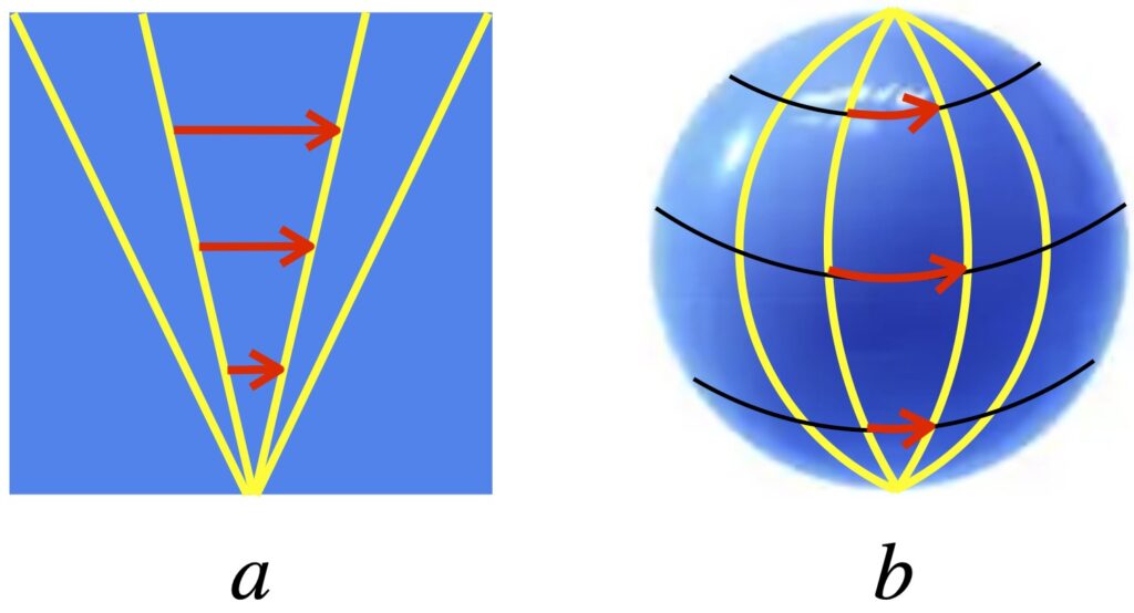
Figure 1a shows a vector field consisting of geodesics (yellow lines). We’ll call this vector field . We can represent the separation between these geodesics by the vectors shown in red. They also form a vector field which we’ll call  . We can think of the 3 separation vectors as moving, in time, along a geodesic. The separation vectors increase in length linearly with time. Thus, we can write:
![\[ \nabla_{\vec{v}} \vec{s} = c \quad \text{(1)} \]](https://www.samartigliere.com/wp-content/ql-cache/quicklatex.com-674be0faf869d50783b79825b8429f3f_l3.png "Rendered by QuickLaTeX.com")
where  is a constant. If we take the second covariant derivative of the expression on the lefthand side of eq. (1) with respect to , we get:
![\[ \nabla_{\vec{v}} \nabla_{\vec{v}} \vec{s} = 0 \quad \text{(2)} \]](https://www.samartigliere.com/wp-content/ql-cache/quicklatex.com-3af55f41a11bcaa616586486b0967457_l3.png "Rendered by QuickLaTeX.com")
since the derivative of a constant is zero.
Contrast this with the situation on a curved space like the surface of a sphere (figure 1b). If we start at the top of the sphere, the separation vector is small. As we move downward, the separation vector gets bigger and bigger until it reaches a maximum at the equator. Then it gets smaller and smaller again. Obviously, because the magnitude of the separation vector are changing, the first derivative of the separation field with respect to is nonzero. However, unlike the case in flat space, the rate at which the separation vectors change as we move along differs. Thus, the second derivative is also nonzero:
![\[ \nabla_{\vec{v}} \nabla_{\vec{v}} \vec{s} \neq 0 \quad \text{(3)} \]](https://www.samartigliere.com/wp-content/ql-cache/quicklatex.com-c0e5489e31bab2a2b199b0f77f9a20ff_l3.png "Rendered by QuickLaTeX.com")
In fact, using the geodesic deviation is an alternative method to the Riemann tensor in determining whether a space is flat or curved. We can quantify this as follows:
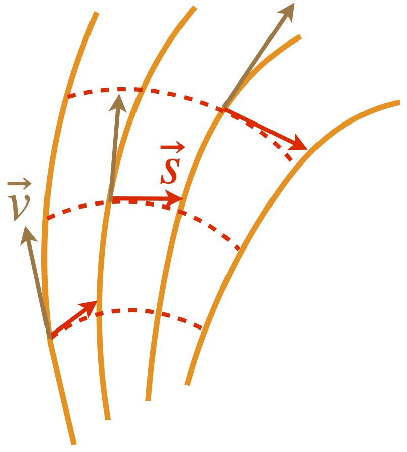
Consider figure 2 which shows: 1) a vector field made of geodesics (field lines depicted in orange; tangent vectors, , depicted in brown) and 2) another vector field created by separation vectors (field lines depicted as red dotted lines; tangent vectors, , represented by solid red arrows).
We know that, by the definition of a geodesic, that:
![\[ \nabla_{\vec{v}} \vec{v} = 0 \quad \text{(4)} \]](https://www.samartigliere.com/wp-content/ql-cache/quicklatex.com-0a84dc1aa2cdd01530db07d359dd4e8f_l3.png "Rendered by QuickLaTeX.com")
Taking the covariant derivative with respect to on both sides, we get:
![\[ \nabla_{\vec{s}} \nabla_{\vec{v}} \vec{v} = 0 \quad \text{(5)} \]](https://www.samartigliere.com/wp-content/ql-cache/quicklatex.com-19d046f551a4272b623ee3fb18a778c3_l3.png "Rendered by QuickLaTeX.com")
We add zero to the left side of eq. (5) in the form  . That gives us:

The and field lines form closed rectangles. Therefore, the Lie bracket ![[\vec{v}, \vec{s}] = \nabla_{\vec{v}} \vec{s} - \nabla_{\vec{s}} \vec{v} = 0](https://www.samartigliere.com/wp-content/ql-cache/quicklatex.com-da62c6b5a9b22e3302b16b9d8252d4c0_l3.png "Rendered by QuickLaTeX.com") which implies that
which implies that  (i.e., we can swap and in the covariant derivative expression. Applying this to eq. (6) yields:

 is called the geodesic deviation. There are other equivalent ways that it can be expressed:

or

We’ll use the form given in eq. (7). And we can use the geodesic deviation to determine if a space is curved or flat.
In figure 3a, we have 2 geodesics in flat space (shown in orange) forming a vector field. Another vector field is formed by the separation vectors between the geodesics (shown in red). In figure 3a, the separation vectors are not changing as we go upward (think of moving upward as moving forward in time). Thus, the derivative of is zero.
On the other hand, in figure 3b – again in flat space – the separation vectors are increasing with time but at a constant rate (i.e., the first derivative of is a constant). However, the second derivative is zero (i.e., the derivative of a constant is zero). That makes the geodesic deviation zero.
Contrast this with geodesics in curved space. Figure 4 shows such geodesics.
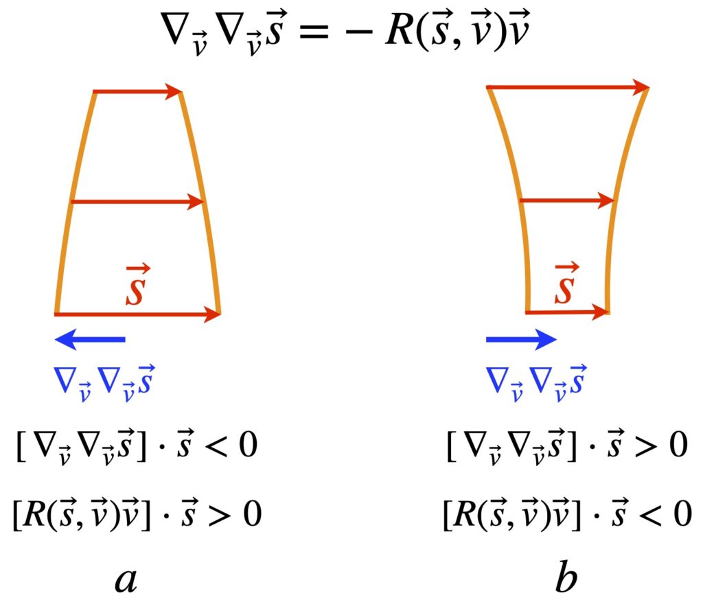
In figure 4a, the geodesics converge as one might see on a spherical surface. The separation vectors, , are decreasing but the rate of this decrease is decreasing meaning the that second derivative is negative (depicted by the blue arrow). If we take the inner product of the geodesic deviation with , it will be negative because (red arrows) and the geodesic deviation (blue arrow) point in different directions. Because the geodesic deviation and the Riemann tensor have different signs, the inner product of the Riemann tensor tensor and is positive.
Figure 4b shows a curved space where geodesics diverge. In this case, the separation vectors are increasing so the first derivative is positive. The rate at which they’re changing is increasing with increasing time (i.e., the upward direction). Thus, the geodesic deviation (i.e. second derivative) is positive. It points in the same direction as so the inner product of the geodesic deviation and is positive. Because the geodesic deviation and the Riemann tensor have different signs, the inner product of the Riemann tensor tensor and is negative.
Sectional Curvature
The inner product of the Riemann tensor with the separation vector tells us whether geodesics in a curved space are converging or diverging. However, this quantity depends on the magnitudes of vectors and . We’d like to us a quantity that’s normalized. We can do this by dividing by the square of the area of the parallelogram formed by and .
Consider the parallelogram shown in figure 5.
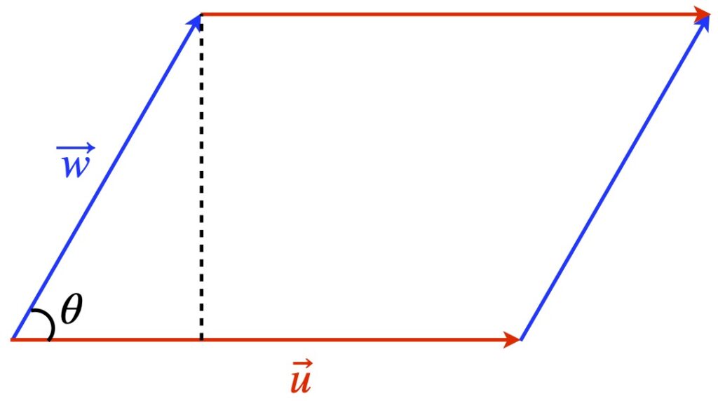
We know that the area of this parallelogram is given by:

Therefore,

To normalize the inner product of the Riemann Curvature Tensor and the separation vector, we divide that entity by eq. (1). What we get is the sectional curvature:
![\[ K(\vec{s}, \vec{v}) = \frac{\bigl[ R(\vec{s}, \vec{v}) \vec{v} \bigr] \cdot \vec{s}}{\bigl( \vec{s} \cdot \vec{s} \bigr) \bigl( \vec{v} \cdot \vec{v} \bigr) - \bigl( \vec{s} \cdot \vec{v} \bigr)^2} \quad \text{(2)} \]](https://www.samartigliere.com/wp-content/ql-cache/quicklatex.com-ef4f1cb065dcb7937a99f68e0c84c3e2_l3.png "Rendered by QuickLaTeX.com")
eigenchris, at 12:35 of the Youtube video Tensor Calculus 24: Ricci Tensor Geometric Meaning (Sectional Curvature) , proves that this relationship holds for any vectors in the plane of and .
Ricci Curvature
From the sectional curvature, we can define the Ricci curvature. We do this by taking an orthonormal basis  and select a direction vector
  . We then define the Ricci curvature in the direction of as the sum of the sectional curvatures along every other basis vector direction aside from . Thus, we can think of the Ricci curvature in the direction of as the average of all possible sectional curvatures containing :
![\[ Ric(\vec{v}, \vec{v}) = \sum_{i=1}^{n-1} K(\vec{\vec{e}_i}, \vec{v}) = \sum_i \frac{\bigl[ R(\vec{e}_i, \vec{v}) \vec{v} \bigr] \cdot \vec{e}_i}{\bigl( \vec{e}_i \cdot \vec{e}_i \bigr) \bigl( \vec{v} \cdot \vec{v} \bigr) - \bigl( \vec{e}_i \cdot \vec{v} \bigr)^2} \quad \text{(1)} \]](https://www.samartigliere.com/wp-content/ql-cache/quicklatex.com-1ca92104b599c09e6e98e7338600ee58_l3.png "Rendered by QuickLaTeX.com")
The geometric interpretation of the Ricci curvature is that it reflects the volume of an object as it flows along geodesics.
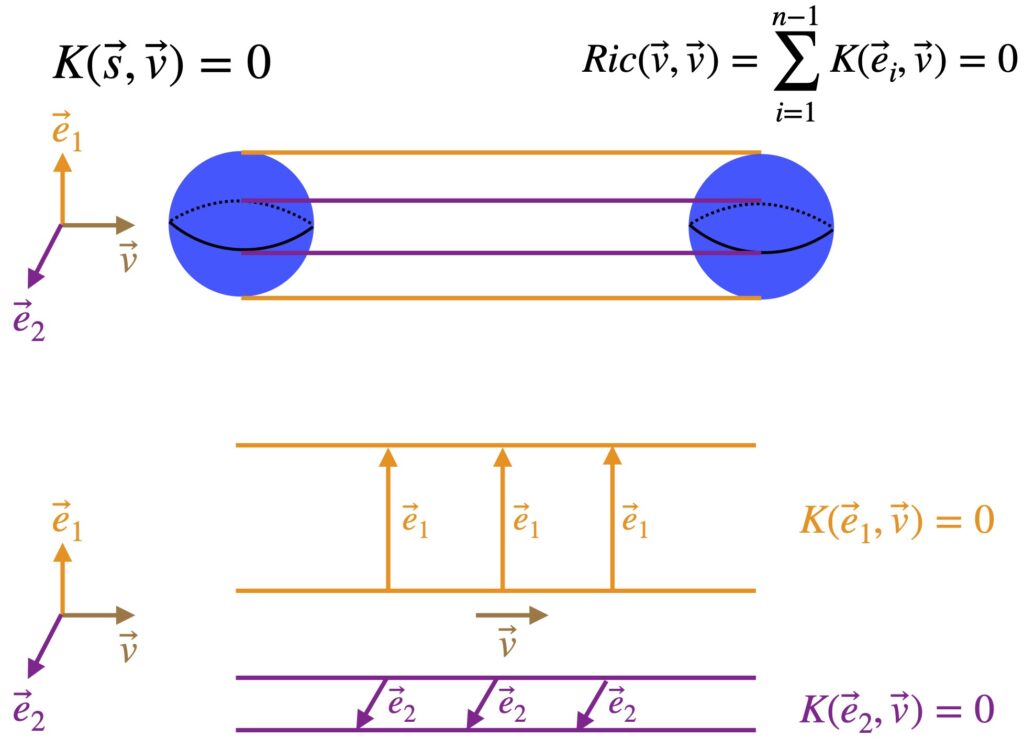
Figure 1 shows a sphere in flat space. Sectional curvature in both the  and
and  directions are zero. Thus, the Ricci curvature, which is the sum of these sectional curvatures, is also zero. In such a setting, the sphere’s volume remains unchanged at all points along the geodesic.
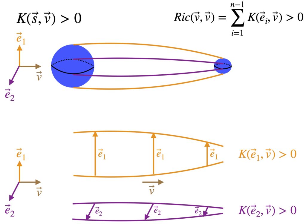
Figure 2 shows a sphere in curved space where geodesics converge. Sectional curvature in both the and directions are positive. Thus, the Ricci curvature is also positive. In this setting, the sphere’s volume decreases from the lefthand portion to the righthand portion of the geodesics.
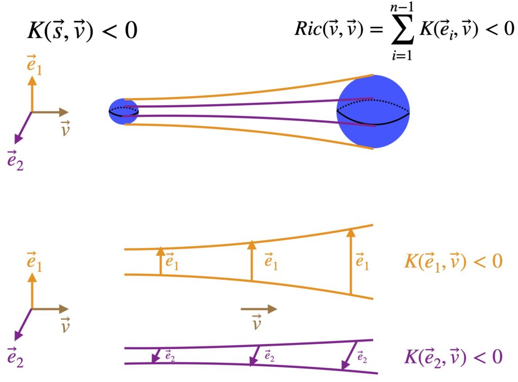
Figure 3 shows a sphere in curved space where geodesics diverge. Sectional curvature in both the and directions are negative. Thus, the Ricci curvature is negative. In this setting, the sphere’s volume increases from the lefthand portion to the righthand portion of the geodesics.
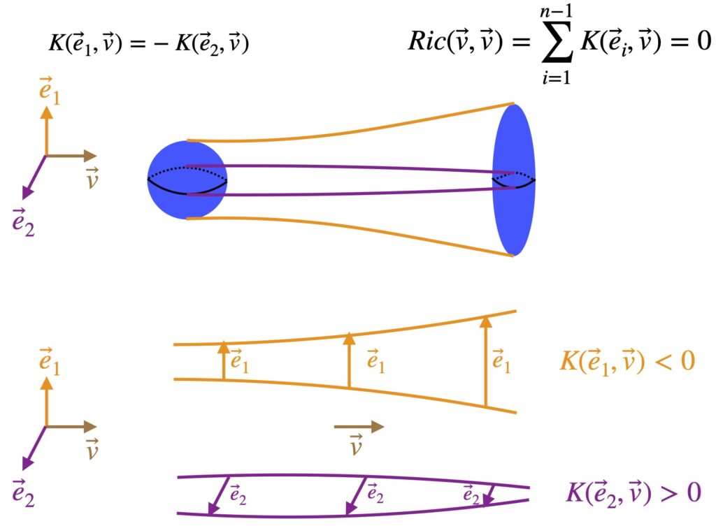
The situation depicted in figure 4 is a bit more complicated. The separation vectors in the direction diverge while the separation vectors in the direction converge. Accordingly, the sectional curvature associated with the direction is negative but the sectional curvature in the direction is positive. In this case, the sectional curvatures in each direction counteract each other, making the Ricci curvature zero. However, this, obviously, is not flat space. Here, the sphere elongates in the in the direction and shortens in the direction but the volume of the sphere remains the same. Thus, the Ricci curvature is can tells us about changes in volume as we move along geodesics but not change in shape.
Note that figures 1-4 contain an error. Since we only have 2 curvature directions, I should have represented the “volume” element changing with geodesics, not as a sphere but as a circular disc – a 2D object. The general arguments given in the explanations, however, still apply.
Our next task is to see how the Ricci curvature relates to the Ricci tensor. Starting with the definition of the Ricci curvature:
![\begin{align*} Ric(\vec{v}, \vec{v}) &= \sum_i \frac{\bigl[ R(\vec{e}_i, \vec{v}) \vec{v} \bigr] \cdot \vec{e}_i}{\bigl( \vec{e}_i \cdot \vec{e}_i \bigr) \bigl( \vec{v} \cdot \vec{v} \bigr) - \bigl( \vec{e}_i \cdot \vec{v} \bigr)^2} \\ &= \sum_i \frac{\bigl[ R(\vec{e}_i, \vec{v}) \vec{v} \bigr] \cdot \vec{e}_i}{\bigl( \underbrace{\cancel{\vec{e}_i \cdot \vec{e}_i}}_{1} \bigr) \bigl( \underbrace{ \cancel{\vec{v} \cdot \vec{v}}}_{1} \bigr) - \bigl( \underbrace{\cancel{\vec{e}_i \cdot \vec{v}}}_{0} \bigr)^2} \\ &= \bigl[ R(\vec{e}_i, \vec{v}) \vec{v} \bigr] \cdot \vec{e}_i \\ &= \bigl[ R(\vec{e}_i, v^j \vec{e}_j) v^k \vec{e}_k \bigr] \cdot \vec{e}_i \\ &= v^j v^k \bigl[ R(\vec{e}_i, \vec{e}_j) \vec{e}_k \bigr] \cdot \vec{e}_i \\ &= v^j v^k R^i_{kij} \\ &= v^j v^k R_{kj} \end{align*}](https://www.samartigliere.com/wp-content/ql-cache/quicklatex.com-69866420ae18c03363fddeced76930de_l3.png "Rendered by QuickLaTeX.com")
 is the Ricci tensor. When the Ricci tensor acts twice on the same vector, we get the Ricci curvature. It can be shown that this is true for any orthonormal basis.
We can generalize the above concepts to any arbitrary basis (not just orthonormal bases) by making use of the volume element derivative. Proof of this can be found at the eigenchris YouTube video Tensor Calculus 25 – Geometric Meaning Ricci Tensor/Scalar (Volume Form).
Note that the only contraction of the Riemann curvature tensor that’s nonzero is the contraction of its first and third indices, the contraction that results in the Ricci tensor.
Ricci Scalar
This discussion is largely taken from the eigenchris YouTube video Tensor Calculus 25 – Geometric Meaning Ricci Tensor/Scalar (Volume Form).
The Ricci scalar is defined as the contraction of the Ricci Tensor with and upper and lower index:
![\[ R = R^i_i = g^{ij} R_{ij} \quad \text{(1)} \]](https://www.samartigliere.com/wp-content/ql-cache/quicklatex.com-eef5a87ab127d1750aceb51b3fbc042b_l3.png "Rendered by QuickLaTeX.com")
The geometric meaning of the Ricci scalar can be thought of as representing how the volume of a ball in curved space deviates from its volume in flat space. This is illustrated in figure 1.
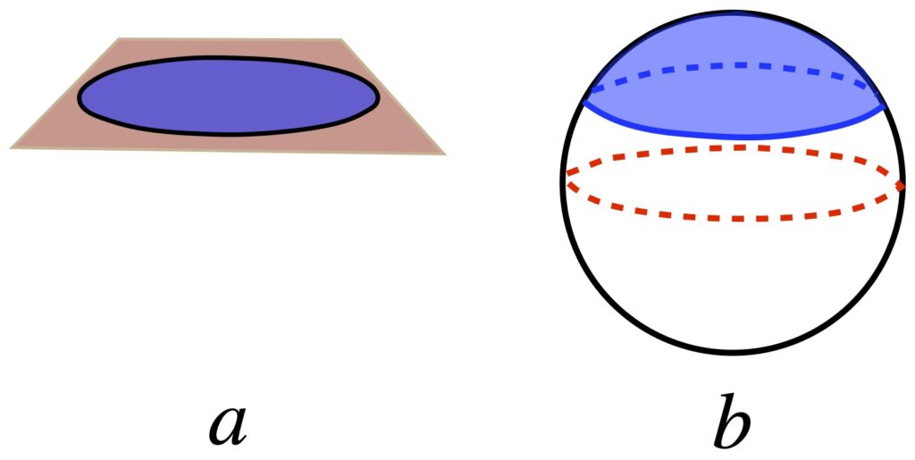
Figure 1a shows a circle with area = A in flat space. A circle of the same circumference in a space with positive curvature has a greater area (figure 1b). In this case, the curved space is a 2D spherical surface and the area that we’re talking about is like a cap at the north pole of the sphere. This idea can be expanded to higher dimensions but visualization in such higher dimensions is more difficult.
On the other hand, for a circle of radius  in flat space, the area of is
  . However, in a positively curved space like the spherical surface shown in figure 1b, a circle of the same radius is less than . (Here, the radius is not the radius from the center of the circular base to the circumference of the circle, but rather, the arc length on the sphere’s cap measured from the north pole to the circumference of the circular base.)
Things are exactly opposite for a negatively curved space like a saddle-shaped 2D space.
These concepts are summarized in the figures below, taken from the eigenchris video cited above.
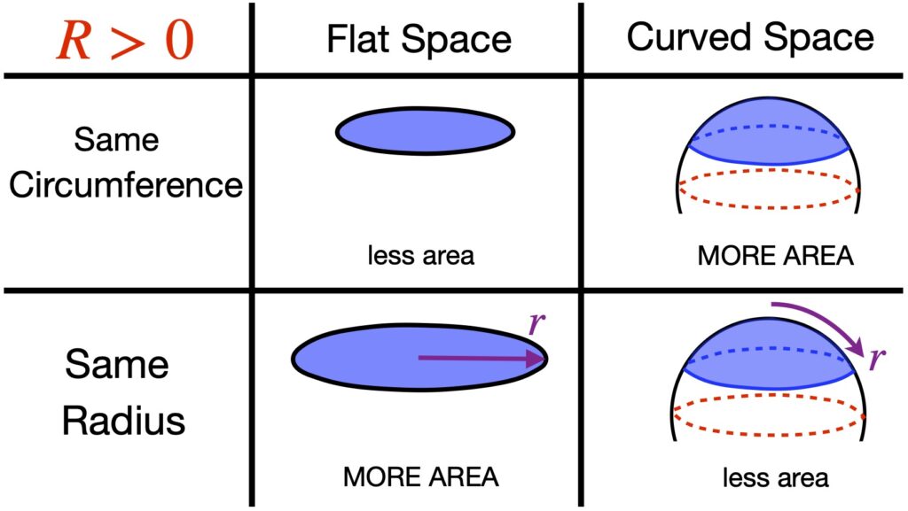
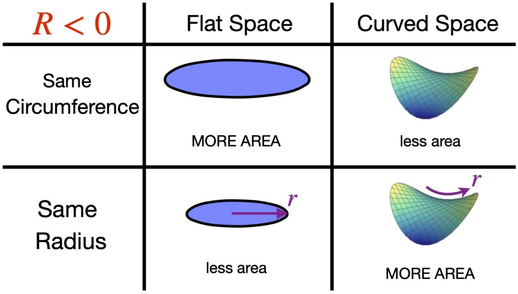
Properties of the Ricci Tensor/Scalar
There are some important properties of the Ricci tensor and scalar that we should discuss. I’ll prove a couple of them but I’ll just state the second Bianchi identity since it’s proof is tedious. However, proof of this identity can be found at 8:43 of the YouTube video by eigenchris, Tensor Calculus 26 – Ricci Tensor/Scalar Properties.
Ricci Tensor Symmetry
![\[ R_{ij} = R{ji} \quad \text{(1)} \]](https://www.samartigliere.com/wp-content/ql-cache/quicklatex.com-5094c2a6ff793fac8356b7932d87b307_l3.png "Rendered by QuickLaTeX.com")
![\[ R^d_{cab} + R^d_{bca} + R^d_{abc} = 0 \]](https://www.samartigliere.com/wp-content/ql-cache/quicklatex.com-6c528056bd6f25f6f78d3217cc206da6_l3.png "Rendered by QuickLaTeX.com")
 . We get:
![\[ R^a_{cab} + R^a_{bca} + \underbrace{\cancel{R^a_{abc}}}_{0} = 0 \]](https://www.samartigliere.com/wp-content/ql-cache/quicklatex.com-42f090c1a225b46597d702a0863b4c4d_l3.png "Rendered by QuickLaTeX.com")
![\[ R^a_{cab} + R^a_{bca} = 0 \]](https://www.samartigliere.com/wp-content/ql-cache/quicklatex.com-40e5706c48eb50d4c19e3464711520d5_l3.png "Rendered by QuickLaTeX.com")
![\[ R_{cb} - R_{bc} = 0 \]](https://www.samartigliere.com/wp-content/ql-cache/quicklatex.com-18693f00bd020c3854b343851e3be19d_l3.png "Rendered by QuickLaTeX.com")
![\[ R_{cb} = R_{bc} \]](https://www.samartigliere.com/wp-content/ql-cache/quicklatex.com-b4432280973dfd1ce43c5945b377a861_l3.png "Rendered by QuickLaTeX.com")
Second Bianchi Identity
![\[ R^d_{cab;i} + R^d_{cia;b} + R^d_{cbi;a} = 0 \quad \text{(2)} \]](https://www.samartigliere.com/wp-content/ql-cache/quicklatex.com-99dcb0eb7cfa64e29eed634338440b5c_l3.png "Rendered by QuickLaTeX.com")
Contracted Bianchi Identity
![\[ \nabla_n \bigl( R^{mn} -\frac12 Rg^{mn} \bigr) = \nabla_n G^{mn} = 0 \quad \text{(3)} \]](https://www.samartigliere.com/wp-content/ql-cache/quicklatex.com-531b6336a6be24c417476d140cab08c4_l3.png "Rendered by QuickLaTeX.com")
![\[ R^d_{bmn;l} + R^d_{blm;n} + R^d_{bnl;m} = 0 \quad \text{(1)} \]](https://www.samartigliere.com/wp-content/ql-cache/quicklatex.com-250b481d0f580a63d9ea5744c0770eff_l3.png "Rendered by QuickLaTeX.com")


![\[ \nabla_{\vec{e}_i} \Bigl( g(R) \Bigr) = \underbrace{\Bigl( \vec{e}_i g \Bigr)}_{0}(R) + g\bigl( \vec{e}_i R \bigr) \]](https://www.samartigliere.com/wp-content/ql-cache/quicklatex.com-4f1d9a245e5fffc7b52ae7c2a15433da_l3.png "Rendered by QuickLaTeX.com")
 (proof
 ![\[ \nabla_{\vec{e}_i} \Bigl( g(R) \Bigr) = g\bigl( \vec{e}_i R \bigr) \]](https://www.samartigliere.com/wp-content/ql-cache/quicklatex.com-f95b51eda19d824e4f9eaff69ed70058_l3.png "Rendered by QuickLaTeX.com")
 and apply the 12 symmetry to the term
  . This changes the sign of these terms:
![\[ g^{bn} \Bigl( R^m_{bmn;l} - R^m_{bml;n} - g^{am} R_{banl;m} \Bigr) = 0 \quad \text{(5)} \]](https://www.samartigliere.com/wp-content/ql-cache/quicklatex.com-0a0113c549cea4fffb5446a75bc722c2_l3.png "Rendered by QuickLaTeX.com")
![\[ \Bigl( R_{bn;l} - R_{bl;n} - g^{am} R_{banl;m} \Bigr) = 0 \quad \text{(6)} \]](https://www.samartigliere.com/wp-content/ql-cache/quicklatex.com-819ba1856ea30af96fcbd8b75a816737_l3.png "Rendered by QuickLaTeX.com")
 to raise the b-indices on the terms in parentheses:
![\[ \Bigl( R^n_{n;l} - R^n_{l;n} - g^{am} R^n_{anl;m} \Bigr) = 0 \quad \text{(7)} \]](https://www.samartigliere.com/wp-content/ql-cache/quicklatex.com-cb6499de29ae3d1bba91a88f9b2c19cc_l3.png "Rendered by QuickLaTeX.com")
 to get another Ricci tensor. Then we raise the a-index of that resulting term to yield:
![\[ \Bigl( R^n_{n;l} - R^n_{l;n} - R^m_{l;m} \Bigr) = 0 \quad \text{(8)} \]](https://www.samartigliere.com/wp-content/ql-cache/quicklatex.com-44c6b3af064aadd9ed801caebe67bc27_l3.png "Rendered by QuickLaTeX.com")
![\[ \Bigl( R^n_{n;l} - R^n_{l;n} - R^m_{l;m} \Bigr) = 0 \quad \text{(9)} \]](https://www.samartigliere.com/wp-content/ql-cache/quicklatex.com-97f294aa2c1e95e01367efa32da28eff_l3.png "Rendered by QuickLaTeX.com")

![\[\frac12 \delta^n_l R_{;n} - R^n_{l;n} = 0 \quad \text{(11)} \]](https://www.samartigliere.com/wp-content/ql-cache/quicklatex.com-68bad7720306bfe3e9510613b7118b05_l3.png "Rendered by QuickLaTeX.com")
 :
:![\[\frac12 g^{ml}\delta^n_l R_{;n} - g^{ml}R^n_{l;n} = 0 \quad \text{(12)} \]](https://www.samartigliere.com/wp-content/ql-cache/quicklatex.com-11943a9fc0ab7eaaba97d7e702487a4f_l3.png "Rendered by QuickLaTeX.com")
![\[\frac12 g^{mn} R_{;n} - R^{mn}_{;n} = 0 \quad \text{(13)} \]](https://www.samartigliere.com/wp-content/ql-cache/quicklatex.com-b3094eb081a270c0b531284ffb05d8db_l3.png "Rendered by QuickLaTeX.com")
![\[ R^{mn}_{;n} - \frac12 g^{mn} R_{;n} = 0 \quad \text{(14)} \]](https://www.samartigliere.com/wp-content/ql-cache/quicklatex.com-0abf8ece02c1e49bb7755316d5c8ae02_l3.png "Rendered by QuickLaTeX.com")
![\[ \nabla_n \Bigl( R^{mn} - \frac12 g^{mn} R \Bigr) = 0 \quad \text{(15)} \]](https://www.samartigliere.com/wp-content/ql-cache/quicklatex.com-482c6ef9a859282b8fbe774ff50a4d8b_l3.png "Rendered by QuickLaTeX.com")
Einstein Field Equation
At the center of general relativity is Einstein’s field equation. It’s what we’ve been working toward and solutions to this equation 1) supply the answer to questions Newtonian gravity cannot answer and 2) provide a description of some of the most interesting phenomena in all of physics.
I’ll present 2 derivations of this equation here. The first follows, in a general way, how Einstein originally arrived at the equation. The second is a derivation from first principles, a derivation based on the principle of stationary action.
Derivation 1
Intuition
We’ve already talked about the geodesic equation, which says that the covariant acceleration along a geodesic is zero:
![\[\frac{d^2 x^{\sigma}}{d\tau^2} + \Gamma^{\sigma}_{\mu \nu} \frac{dx^{\mu}}{d\tau} \frac{dx^{\mu}}{d\tau} =0 \quad\text{(1)}\]](https://www.samartigliere.com/wp-content/ql-cache/quicklatex.com-4ae0a17cfd9091e2787e89a8c1302e6f_l3.png "Rendered by QuickLaTeX.com")
so
![\[\frac{d^2 x^{\sigma}}{d\tau^2} = -\Gamma^{\sigma}_{\mu \nu} \frac{dx^{\mu}}{d\tau} \frac{dx^{\mu}}{d\tau} \quad \text{(2)} \]](https://www.samartigliere.com/wp-content/ql-cache/quicklatex.com-5a0f98fb1216f23abb3149d2a117a22c_l3.png "Rendered by QuickLaTeX.com")
In non relativistic physics, Newton’s second law is:
![\[ F=ma = mg \quad \Rightarrow \quad a = g =\frac{F}{m} \quad \text{(3)}\]](https://www.samartigliere.com/wp-content/ql-cache/quicklatex.com-5548b20fcc279941ece06d28d998200d_l3.png "Rendered by QuickLaTeX.com")
where is the acceleration due to gravity of the earth.
Let’s assume our mass is a unit mass (i.e.  ). Then:
![\[ a = F \quad \text{(4)} \]](https://www.samartigliere.com/wp-content/ql-cache/quicklatex.com-4210229ac51f643471d9d2696621c5a1_l3.png "Rendered by QuickLaTeX.com")
We know that 
Thus:
![\[\frac{d^2 x}{dt^2} = F \quad \text{(6)} \]](https://www.samartigliere.com/wp-content/ql-cache/quicklatex.com-2126854558947820266652c2596f0d23_l3.png "Rendered by QuickLaTeX.com")
If we compare the Newtonian equation, eq. (6), with the geodesic equation, eq. (2), we can see a similarity. On the left side of both equations are acceleration terms. On the righthand side of the geodesic equation is a term containing the Christoffel symbol that we can consider analogous to a force.
Any relativistic theory of gravity should reduce to the Newtonian gravitation. Thus, we can see what happens to eq (2) under the non relativistic conditions in which Newtonian gravitation is applicable. These conditions are:
- Speeds are slow (i.e.,
 )
) - Gravity is weak (i.e., we can consider it a perturbation of flat space)
- The gravitational field is static (i.e., unchanging with time)
Condition 1 means that velocities in the spatial directions are negligible compared to velocity in the time direction, which is the speed of light. Thus,
![\[ \frac{dx^i}{d\tau} \ll \frac{dt}{d\tau} \quad \text{(7)} \]](https://www.samartigliere.com/wp-content/ql-cache/quicklatex.com-947771e810c0f1a982a3d36fcaba1e56_l3.png "Rendered by QuickLaTeX.com")
Therefore:
![\[\frac{d^2 x^{\sigma}}{d\tau^2} + \Gamma^{\sigma}_{\mu \nu} \frac{dx^{\mu}}{d\tau} \frac{dx^{\mu}}{d\tau} =0 \quad \Rightarrow \quad \frac{d^2 x^{\sigma}}{d\tau^2} + \Gamma^{\sigma}_{00} \frac{dt}{d\tau}^2 =0 \quad\text{(8)} \]](https://www.samartigliere.com/wp-content/ql-cache/quicklatex.com-d053433d4033d4e514d2e705e741b701_l3.png "Rendered by QuickLaTeX.com")
Next, it’s known from special relativity that:
![\[ \frac{dt}{d\tau} = \gamma = \frac{1}{\sqrt{1-\frac{v^2}{c^2}}} \quad\text{(9)} \]](https://www.samartigliere.com/wp-content/ql-cache/quicklatex.com-5069edba8a3389e9bc283f320b21698b_l3.png "Rendered by QuickLaTeX.com")
But  . So,
. So,  and therefore:
![\[ \frac{dt}{d\tau} \approx 1 \quad\text{(10)} \]](https://www.samartigliere.com/wp-content/ql-cache/quicklatex.com-e61ca5c72154b714f94e2e1167682989_l3.png "Rendered by QuickLaTeX.com")
This makes eq. (8):
![\[ \frac{d^2 x^{\sigma}}{d\tau^2} + \Gamma^{\sigma}_{00} =0 \quad\text{(11)} \]](https://www.samartigliere.com/wp-content/ql-cache/quicklatex.com-adafc380bb1a5c631de3b8310726a331_l3.png "Rendered by QuickLaTeX.com")
 also implies that
  . Thus:
![\[ \frac{d^2 x^{\sigma}}{dt^2} + \Gamma^{\sigma}_{00} =0 \quad\text{(11)} \]](https://www.samartigliere.com/wp-content/ql-cache/quicklatex.com-58e897b969e4d4543549d49f77d445ee_l3.png "Rendered by QuickLaTeX.com")
If we let  ,
,  . Then
  . Thus:

which implies that
![\[ \Gamma^0_{00} = 0 \]](https://www.samartigliere.com/wp-content/ql-cache/quicklatex.com-1edae6e136b6667b93cc1545ed31864f_l3.png "Rendered by QuickLaTeX.com")
This means that the only nonzero Christoffel symbols are those where  (i.e.,
  .
.
So eq. (11) becomes:
![\[ \frac{d^2 x^i}{dt^2} + \Gamma^i_{00} =0 \quad\text{(12)} \]](https://www.samartigliere.com/wp-content/ql-cache/quicklatex.com-cb063ce5dc5ab6438303550e8fc306b7_l3.png "Rendered by QuickLaTeX.com")
Expressing  in terms the metric, we have:
![\[ \Gamma^i_{00} = \frac12 g^{i \lambda}\bigl( \partial_0 g_{ \lambda 0} + \partial_0 g_{0 \lambda} - \partial_{\lambda} g_{00}\bigr) \quad\text{(13)} \]](https://www.samartigliere.com/wp-content/ql-cache/quicklatex.com-3edc90466d9e45a7e1a717eb1d1c81b6_l3.png "Rendered by QuickLaTeX.com")
Because the field is static, the metric isn’t changing which means that the time derivatives of the metric are zero. Therefore:
![\[ \Gamma^i_{00} = \frac12 g^{i \lambda} \partial_{\lambda} g_{00} \quad\text{(14)} \]](https://www.samartigliere.com/wp-content/ql-cache/quicklatex.com-3ee7015a54c46eee567eb1b84ec3fd77_l3.png "Rendered by QuickLaTeX.com")
Now the second condition under which we’re operating (i.e., the gravitational field is weak) means that we can decompose the metric into the Minkowski metric plus a small perturbation:
![\[ g_{\mu \nu} = \eta_{\mu \nu} + h_{\mu \nu} \quad\text{(15)} \]](https://www.samartigliere.com/wp-content/ql-cache/quicklatex.com-ddaa97017e14b6fb97cea20362557744_l3.png "Rendered by QuickLaTeX.com")
We need to find an expression for the inverse metric that we can use in eq. (14). We can do this as follows:
![\[ \bigl( n^{\alpha \mu} - h^{\alpha \mu} \bigr) \bigl( n_{\mu \nu} + h_{\mu \nu} \bigr) &= g^{\alpha \mu}g_{\mu \nu} = \delta^{\alpha}_{\nu} \quad\text{(16)} \]](https://www.samartigliere.com/wp-content/ql-cache/quicklatex.com-9791b1ad3f04294fbe637721c5e1c4df_l3.png "Rendered by QuickLaTeX.com")
![\[ \underbrace{n^{\alpha \mu} n_{\mu} \nu}}_{\delta^{\alpha}_{\mu}} + \cancel{n^{\alpha \mu} h_{\mu \nu}} - \cancel{h^{\alpha \mu} n_{\mu \nu}} - \underbrace{h^{\alpha \mu} h_{\mu \nu}}_{h^2=0} &= g^{\alpha \mu}g_{\mu \nu} = \delta^{\alpha}_{\nu} \]](https://www.samartigliere.com/wp-content/ql-cache/quicklatex.com-63bb4f289af548e82828624c71a22b33_l3.png "Rendered by QuickLaTeX.com")
To see why  , click .
![\[ n^{\alpha \cancel{\mu}} h_{\cancel{\mu} \nu}} - h^{\alpha \cancel{\mu}} n_{\cancel{\mu} \nu}\]](https://www.samartigliere.com/wp-content/ql-cache/quicklatex.com-e65a4d2716806b98a6aa2b956dd96157_l3.png "Rendered by QuickLaTeX.com")
![\[ n^{\alpha} h_{\mu} - h^{\alpha} n_{\mu}\]](https://www.samartigliere.com/wp-content/ql-cache/quicklatex.com-152de3c40949f494d4c3b6bd8909c650_l3.png "Rendered by QuickLaTeX.com")
![\[ \delta^{\mu}_{\cancel{\alpha}} n^{\cancel{\alpha}} h_{\mu} - \delta^{\mu}_{\cancel{\alpha}} h^{\cancel{\alpha}} n_{\mu} \]](https://www.samartigliere.com/wp-content/ql-cache/quicklatex.com-503aae1134fe1c69c78fe8392559d898_l3.png "Rendered by QuickLaTeX.com")
![\[ n^{\mu} h_{\mu}} - h^{\mu} n_{\mu}} \]](https://www.samartigliere.com/wp-content/ql-cache/quicklatex.com-156c8443e56b265a96099298735228f6_l3.png "Rendered by QuickLaTeX.com")
![\[ n \cdot h - h \cdot n \]](https://www.samartigliere.com/wp-content/ql-cache/quicklatex.com-bcdef365cefb56633a78d61b98e69bd1_l3.png "Rendered by QuickLaTeX.com")
![\[ 0 \]](https://www.samartigliere.com/wp-content/ql-cache/quicklatex.com-736567bf298f1038c64838133a5bad67_l3.png "Rendered by QuickLaTeX.com")
Looking at eq. (16), we can equate the terms  and
and 
Renaming indices and recognizing the symmetry of the Minkowski metric and metric tensor, we get:
![\[ g^{\mu \nu} = n^{ \mu \nu} - h^{ \mu \nu} \quad\text{(17)} \]](https://www.samartigliere.com/wp-content/ql-cache/quicklatex.com-dc22e5d45b95b5c619fd05f8b384ed0f_l3.png "Rendered by QuickLaTeX.com")
We then have:

So:

Putting the results of eq. (18) into eq. (14), we get:

All of the spatial terms in the Minkowski metric equal 1 so eq. (19) becomes:
![\[ \Gamma^i_{00} = -\frac12 \partial_i h_{00} \quad\text{(20)} \]](https://www.samartigliere.com/wp-content/ql-cache/quicklatex.com-319b59399a8447359a8a101e6d1ab98a_l3.png "Rendered by QuickLaTeX.com")
Substituting eq. (20) into eq. (12) gives us:

What this means is that, in Newtonian gravitational theory, the acceleration tells an object how to move. In general relativity, however, the thing that tells an object how to move is curvature of spacetime (which in eq. (21) is represented by the small perturbation of the metric tensor,  ).
).
We can continue this line of thought by noting that, in Newtonian gravity, for a unit mass:
![\[ \frac{d^2x^i}{dt^2} = a = F = -\nabla \phi \quad \text{(22)} \]](https://www.samartigliere.com/wp-content/ql-cache/quicklatex.com-d5456c624246a6a1f89ff379dc8a6525_l3.png "Rendered by QuickLaTeX.com")
But we just saw that, in the Newtonian limit of general relativity:
![\[ a = \frac12 \partial_i h_{00} \quad \text{(23)} \]](https://www.samartigliere.com/wp-content/ql-cache/quicklatex.com-f25834a02ace3da0d3c7980caf3ea965_l3.png "Rendered by QuickLaTeX.com")
Therefore:

where  is a constant of integration.
It’s well-known that Poisson’s equation is the field equation of Newtonian gravity:
![\[ \nabla^2 \phi = 4 \pi G \rho (x,t) \quad \text{(25)} \]](https://www.samartigliere.com/wp-content/ql-cache/quicklatex.com-ea13543fb69be052d166a2b3fc12a464_l3.png "Rendered by QuickLaTeX.com")
where
 is the Laplacian operator, an operator that takes 2 spatial derivatives of whatever it operates on
 is the gravitational field
 is the mass density which is a function of space and time
Derivation and solution of eq. (25) can be found here.
Substituting the value for obtained in eq. (24) into eq. (25) yields:

In eq. (26), we begin to see the beginnings of what a field equation in general relativity might look like:
![\[ \text{spacetime curvature } \propto \text{ mass density} \quad \text{(27)} \]](https://www.samartigliere.com/wp-content/ql-cache/quicklatex.com-e5c8363bcb3ea90b634a27274a9f3676_l3.png "Rendered by QuickLaTeX.com")
There’s a problem with eq. (26) though; it’s not a tensor equation. We know the laws of physics need to hold in all coordinate systems. The only way to make this happen is to express these laws with tensor equations. Our goal for the rest of this derivation is to convert eq. (26) into a tensor equation and to generalize this tensor equation so it applies to all conditions, not just to conditions where Newtonian mechanics are valid.
The first dilemma we encounter is that mass density, itself, is not tensorial. Why? Because the mass density differs in differing reference frames. Figure 1 illustrates such a situation.
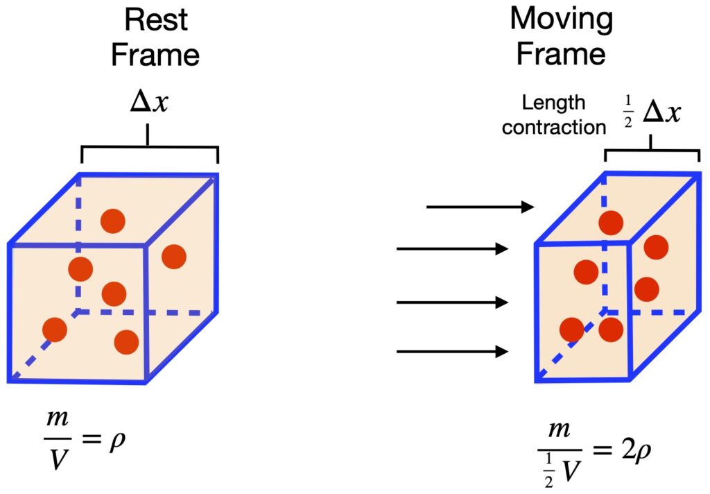
In the diagram, an observer A, in the rest frame of a box of particles, sees a mass density of  where is mass, is volume and
  is the density. However, an observer B, moving to the left with respect to the box, because of length contraction, sees the volume of the box decrease by one-half. Therefore, he sees the mass density of the box as 2 times that noted by observer A:
  . But it’s the same box; this should not be.
The answer to this conundrum is to somehow make the mass density a tensor. In special relativity, the manner in which non-tensor quantities were made into 1-tensors that are invariant under Lorentz transformations was to make them into 4-vectors. Furthermore, it’s worth noting that mass is but one component of the 4-momentum:
![\[ P^u = \left( \frac{E}{c}, p_x, p_y, p_z \right) \quad \text{(1)} \]](https://www.samartigliere.com/wp-content/ql-cache/quicklatex.com-cbc7d9ab4aca35ef7fa6376d39ac2803_l3.png "Rendered by QuickLaTeX.com")
where  . It makes sense, then, that use of this fact might play a role in developing a tensor for mass density. Indeed, this is the case. The tensor that’s found on the right side of the Einstein field equation, the energy-momentum tensor, describes the flow of each component of the 4-momentum in each direction of spacetime. In what follows, we’ll offer a more detailed account of the energy-momentum tensor.
Energy-Momentum Tensor
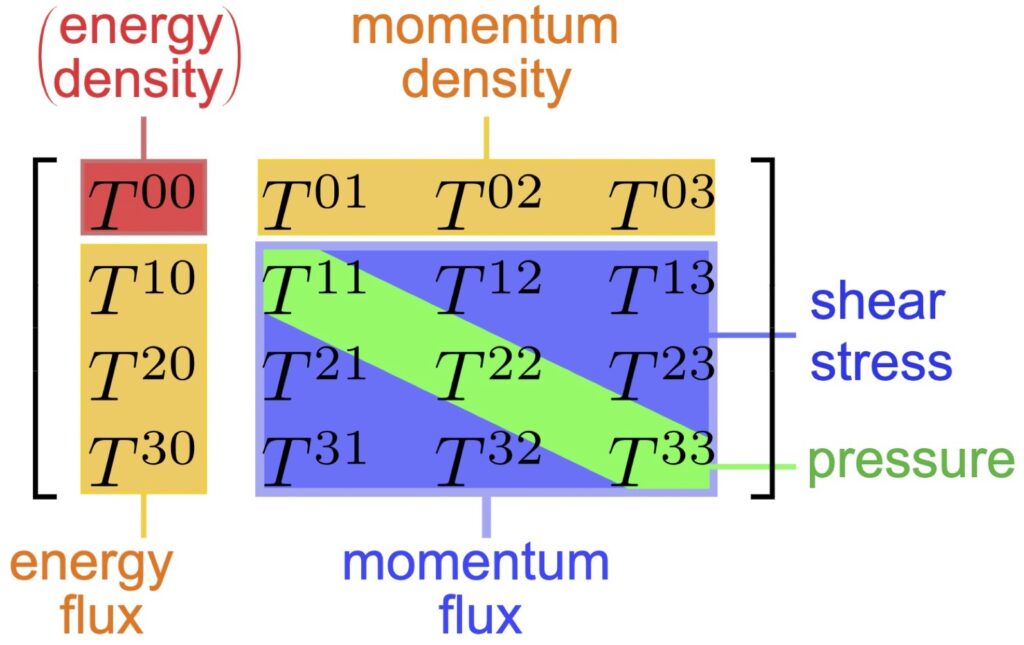
Figure 1 depicts the energy-momentum tensor. The remainder of this section will be devoted to explaining what it means. The derivation that follows is taken largely from the YouTube video by dXoverdteqprogress, Energy-momentum tensor.
Suppose we have have a cluster of particles that don’t interact with each other but which are all moving with the same velocity,  .
.
The number of particles per unit volume is given by:
![\[ n_0 = \frac{N}{V} \quad \text{(1)} \]](https://www.samartigliere.com/wp-content/ql-cache/quicklatex.com-97432c95a1c8242cf83662750d009558_l3.png "Rendered by QuickLaTeX.com")
where  is the number density and
  is the number of particles in volume .
We saw above that, because of length contraction, observer A, who measures the number density of our particle cluster in his own rest frame as  will measure the cluster’s number density, when it’s moving relative to him, as:
![\[ n = \frac{N}{V}\Gamma = n_0 \Gamma \quad \text{(2)} \]](https://www.samartigliere.com/wp-content/ql-cache/quicklatex.com-85f6a76deb2253f79e214bea383aea98_l3.png "Rendered by QuickLaTeX.com")
We define current as the flow of “stuff” across a unit surface per unit time:
![\[ J^i = \rho v^i \quad \text{(3)} \]](https://www.samartigliere.com/wp-content/ql-cache/quicklatex.com-8313583d909a50037d420ad204621695_l3.png "Rendered by QuickLaTeX.com")
where  is the ith component of current,
  is the number density of the “stuff”, and
  is the ith component of the velocity at which the “stuff” is flowing.
The mass density  is given by the particle number density times the mass, , of each particle (which is assumed to be the same for all the particles):
![\[ \epsilon = n_0 m \quad \text{(4)} \]](https://www.samartigliere.com/wp-content/ql-cache/quicklatex.com-ff87da234420fce5aaaa95614c8d83e3_l3.png "Rendered by QuickLaTeX.com")
When special relativity is considered, eq. (4) becomes:
![\[ \epsilon_{\text{Rel}} = n_0 m \gamma^2 \quad \text{(5)} \]](https://www.samartigliere.com/wp-content/ql-cache/quicklatex.com-4d495eade0bd46bf0077117ea2be90b1_l3.png "Rendered by QuickLaTeX.com")
Notice that we have 2 factors of in eq. (5): one due to length contraction and one due to relativistic increase in mass in the moving frame.
Now, the time component of the 4-velocity equals :
![\[ u^0 = \frac{dt}{d\tau} = \gamma \quad \text{(6)} \]](https://www.samartigliere.com/wp-content/ql-cache/quicklatex.com-d880019b14bd55b5b7bb99cf4ed89408_l3.png "Rendered by QuickLaTeX.com")
Substituting eq. (6) into eq. (5), we get:
![\[ \epsilon_{\text{Rel}} = n_0 m u^0 u^0 \quad \text{(7)} \]](https://www.samartigliere.com/wp-content/ql-cache/quicklatex.com-570d42bceb75f1ca7a08536be94dfecd_l3.png "Rendered by QuickLaTeX.com")
From now on, since we are working with relativistic physics, we’ll drop the “Rel” subscript on and simply take  .
.
So, combining the current equation, eq. (3), with eq. (7), we find that the flow of energy per unit time across a unit surface perpendicular to the ith component of space (which is also referred to as energy flux,  ) is:
) is:

We note the following relationships involving the 4-velocity:
![\[ u^0 = \frac{dt}{d\tau} = \gamma \]](https://www.samartigliere.com/wp-content/ql-cache/quicklatex.com-147fc0047e7b715f818485514efa6051_l3.png "Rendered by QuickLaTeX.com")
![\[ u^i = \frac{dx^i}{d\tau} \frac{dt}{dt} = \frac{dx^i}{dt} \frac{dt}{d\tau} = \gamma v^i = u^0 v^i \quad \text{(9)} \]](https://www.samartigliere.com/wp-content/ql-cache/quicklatex.com-558fc6b674c9611f486b6cdec60ec5e6_l3.png "Rendered by QuickLaTeX.com")
Substituting eq. (9) into eq. (8), we have:
![\[ \sigma^i = n_0 m u_0 u_i \quad \text{(10)} \]](https://www.samartigliere.com/wp-content/ql-cache/quicklatex.com-d666067dd3c965f88901393a9cbf81e9_l3.png "Rendered by QuickLaTeX.com")
We know that energy cannot be created or destroyed. Thus, the energy density in a given volume must decrease if net energy is leaving the volume through the “surfaces” of the volume, or increase if net energy enters the volume through its “surfaces.” The equation that describes this concept is called the continuity equation:
![\[ \frac{\partial \epsilon}{\partial t} + \nabla \cdot \vec{\sigma^i} = 0 \quad \text{(11)} \]](https://www.samartigliere.com/wp-content/ql-cache/quicklatex.com-a0ea50d3ed1733cea682208004f5ce80_l3.png "Rendered by QuickLaTeX.com")
which can be written as:
![\[ \frac{\partial \epsilon^i}{\partial x^i} = 0, \quad \epsilon^i = (\epsilon, \sigma^1, \sigma^2, \sigma^3 ) \quad \text{(12)} \]](https://www.samartigliere.com/wp-content/ql-cache/quicklatex.com-4e41281d3c9c510ca57158220ac7bc81_l3.png "Rendered by QuickLaTeX.com")
In eq. (12), is the flow of energy in the time direction (i.e., across a surface perpendicular to the ct-axis). This means that there is no velocity in the spatial directions (i.e., the clump of energy per unit volume we’re talking about is at rest); which means that is just the energy density. The  terms, on the other hand, represent the flow of energy in the i-direction (i.e., across a surface perpendicular to the i-axis).
We can make a similar analysis for each of the components of momentum.
Momentum density,  , is given by:
![\[ P^i = n_o m v^i \gamma^2 = n_o m \underbrace{v^i u^0}_{u^i} u^0 = n_0 m u^i u^0 \quad \text{(13)} \]](https://www.samartigliere.com/wp-content/ql-cache/quicklatex.com-a8d356d859302d9cfcaa9190c69d19d6_l3.png "Rendered by QuickLaTeX.com")
where  is the momentum of the particles in the i-direction. The ith component of momentum density, , traversing a surface perpendicular to the jth spatial direction, then, is:
![\[ P^{ij }= P^i v^j = n_0 m u^i \underbrace{u^0 v^j}_{u^j} = n_0 m u^i u^j \quad \text{(14)} \]](https://www.samartigliere.com/wp-content/ql-cache/quicklatex.com-31f1612d878415ff3c87bb23bded05a7_l3.png "Rendered by QuickLaTeX.com")
We can write a continuity equation for momentum, just as we did for energy:
![\[ \frac{\partial P^i}{\partial t} + \nabla \cdot \vec{P}^i = 0 \quad \text{(15)} \]](https://www.samartigliere.com/wp-content/ql-cache/quicklatex.com-85962b04f28b6a35673c2497d7855df1_l3.png "Rendered by QuickLaTeX.com")
which can be written as:
![\[ \frac{\partial P^i}{\partial x^j} = 0, \quad P^{i j}= (P^i, P^{i1}, P^{i2}, P^{i3} ) \quad \text{(16)} \]](https://www.samartigliere.com/wp-content/ql-cache/quicklatex.com-3e309299fe61a4dd075e152b63d76d57_l3.png "Rendered by QuickLaTeX.com")
To summarize, we have:
| Entity | Physical Meaning | Equations |
| Energy (E) density | Flow of E in time () direction |  |
| Energy (E) flux | Flow of E in spatial ( ) directions ) directions |  |
| Momentum (P) density | Flow of P in time () direction |  |
| Momentum flux (P) | Flow of P in spatial () directions |  |
At this point, we can put the elements that we derived into matrix form.
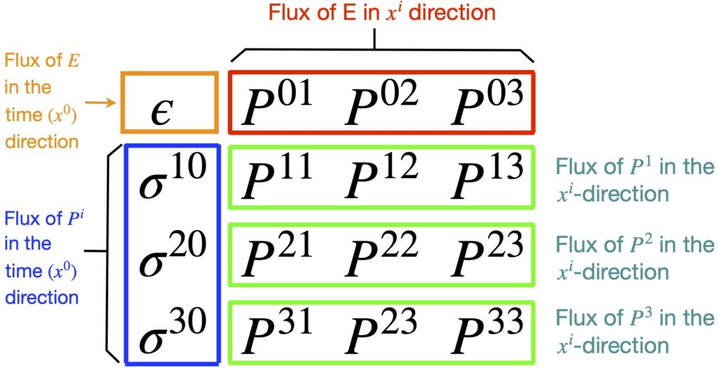
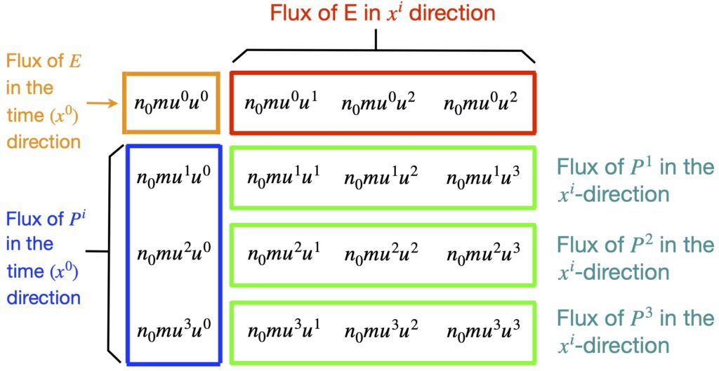
Symmetry
The energy-momentum tensor is symmetric. In what follows, I’ll provide some intuition as to why this is so. This discussion is patterned after
Schutz, Bernard. A First Course in General Relativity. Second ed., Cambridge University Press, 2009, pp. 97-8.
Toi = Tio symmetry
The energy flux terms and momentum density terms are symmetric. We can see this in the following way:
- In special relativity, energy is equivalent to mass:

- Energy density is energy per unit volume:

- Energy flux is given by energy density times volume:
 where is the velocity in direction
 - But momentum times velocity in direction equals momentum in direction :

- Therefore,
![\[ \displaystyle \underbrace{\frac{E}{Vol} \cdot v^i }_{\text{Energy flux}}\,\,\,=\,\,\, \frac{m}{Vol} \cdot v^i \,\,\,= \underbrace{\frac{P^i}{Vol}}_{\substack{\text{Momentum } \\ \text{density}}} \quad \text{(1)} \]](https://www.samartigliere.com/wp-content/ql-cache/quicklatex.com-a4b83affd41acbcfb34680964266443d_l3.png "Rendered by QuickLaTeX.com")
Tij – Tji symmetry
Understanding why the stress terms of the energy-momentum tensor are symmetric is more difficult.
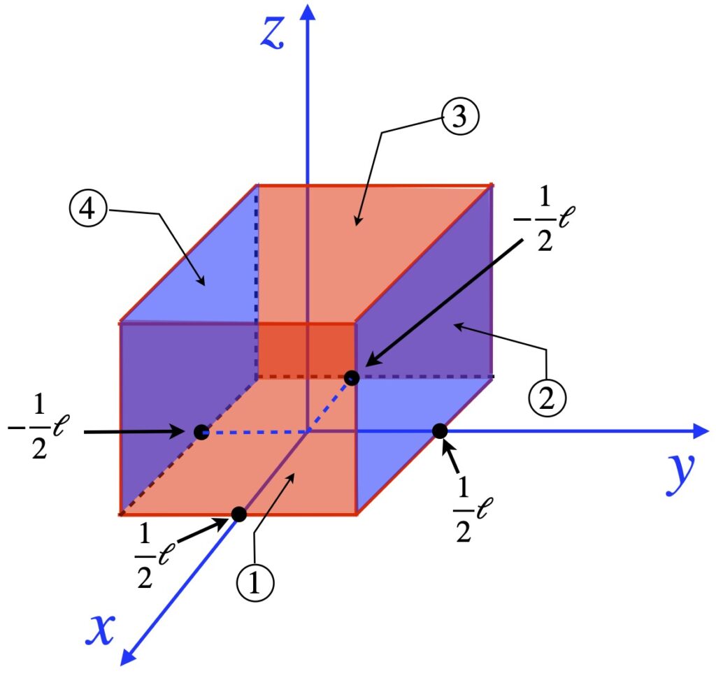
Consider the cube-shaped element with sides of (very small) length  , as shown in figure 1. We will consider forces on the sides labeled 1, 2, 3 and 4. The force by the element on an adjacent element due to flow across side 1 is given by
  where
where  is the area of the surface. Likewise, the force by the element through side 2 on an adjacent element is
  . Here, runs from 1-3 because
  is not necessarily perpendicular to the surface under consideration. Because the force associated with flow through side 1 is in the +x-direction, flow (and thus force) through side 3 (the side opposite side 1) must be be in the opposite direction. Thus,
  . Similarly,
  .
.
Since our element experts forces on its surroundings, its surroundings expert equal and opposite forces on our element. Thus, the forces on each face of our cubic element are  ,
,  ,
,  and
and 
Next, let’s calculate the torque on the cube generated by each of these forces. The torque due to is  . By similar reasoning, the torques related to forces on other faces of the cube are:


We add all of these to get the total torque,  :
:

The moment of inertia,  , is proportional to
  where is mass and is the moment arm – the radius from the origin of the axis we’re rotating about and the point where the force giving rise to torque resides, so we have:
![\[ I = \alpha m \ell^2 = \alpha \frac{m}{\ell^3} \cdot \ell^3 \cdot \ell^2 = \alpha \rho \ell^5 \quad \text{(3)} \]](https://www.samartigliere.com/wp-content/ql-cache/quicklatex.com-bcaeedf645f996f3024b9e43561e431c_l3.png "Rendered by QuickLaTeX.com")
The angular momentum,  , created by the total torque is:
![\[ \ddot \theta = \frac{\tau_{\text{tot}} }{I} = \frac{ \ell^3 \Bigl( T^{xy} - T^{yx} \Bigr)}{\ell^5} = \frac{T^{xy} - T^{yx}}{\alpha \rho \ell^2} \quad \text{(4)} \]](https://www.samartigliere.com/wp-content/ql-cache/quicklatex.com-9c9cf4e2656ce44ace29762a085767f9_l3.png "Rendered by QuickLaTeX.com")
As goes to zero, goes to infinity. But this makes no physical sense; we don’t see fluid elements whirling around inside fluids at infinite speeds. The only way this can be avoided is to say:
![\[ T^{xy} - T^{yx} = 0 \quad \Rightarrow \quad T^{xy} = T^{yx} \quad \text{(5)} \]](https://www.samartigliere.com/wp-content/ql-cache/quicklatex.com-11d39a4afa44da951ff5e78cd2eb06e7_l3.png "Rendered by QuickLaTeX.com")
Therefore, the stress components of the energy-momentum tensor are symmetric.
Note that, although I understand the overall plan of the argue, I have a hard time visualizing where the author is putting his lever arms and where the forces are acting to arrive at the outcome at which he arrives. But then, I was never very good at torque problems. If anyone can enlighten me, please leave a comment via the contact page.
Types
There are a couple of important forms of the energy-momentum tensor that are commonly encountered: dust and a perfect fluid. We’ll discuss each in turn.
Dust
Dust is a collection of non-interacting particles at rest with respect to each other (although the collection might be moving with some velocity, called the drift velocity). Because the particles are at rest in this frame of reference (referred to as the momentarily comoving rest frame – MRCF). Being at rest means the particles have no velocity; which means  . Given this, looking at figure 3, we can see that the only term that’s nonzero is
  . This is the
  component of the energy-momentum tensor. So the energy-momentum tensor of dust is:
![\[\begin{pmatrix} pc^2 & 0 & 0 & 0 \\ 0 & 0 & 0 & 0 \\ 0 & 0 & 0 & 0 \\ 0 & 0 & 0 & 0 \\ \end{pmatrix}\]](https://www.samartigliere.com/wp-content/ql-cache/quicklatex.com-552e13e1a61b3e40931cb005788ed001_l3.png "Rendered by QuickLaTeX.com")
Perfect Fluid
A perfect fluid is one in which particles within a fluid element move randomly in all directions. This creates pressure but there is no heat conduction (i.e., no energy flux and no momentum density;  ) and no viscosity (meaning there are no shear stress forces, and thus, no terms where
  with
with  ). There is however, energy density and pressure (i.e., terms were with
  ). Without providing a detailed derivation, the energy-momentum tensor for a perfect fluid is:
![\[\begin{pmatrix} \rho c^2 & 0 & 0 & 0 \\ 0 & P & 0 & 0 \\ 0 & 0 & P & 0 \\ 0 & 0 & 0 & P \\ \end{pmatrix}\]](https://www.samartigliere.com/wp-content/ql-cache/quicklatex.com-4e85e7c77f3ef565c44c168c04f83032_l3.png "Rendered by QuickLaTeX.com")
An equation that summarizes the energy-momentum tensor of a perfect fluid is:
![\[ T^{\mu \nu} = \bigl( \rho + \frac{P}{c^2} \bigr) U^{\mu} U^{\nu} - P \eta^{\mu \nu} \quad \text{(1)} \]](https://www.samartigliere.com/wp-content/ql-cache/quicklatex.com-98ee008157a45648605193a313c83509_l3.png "Rendered by QuickLaTeX.com")
To see this, consider the case of dust. We know that In the MCRF
![\[ U^u = 1,0,0,0 \quad \text{(2)} \]](https://www.samartigliere.com/wp-content/ql-cache/quicklatex.com-477770bfed2fdd812850116cb2e28255_l3.png "Rendered by QuickLaTeX.com")
Where there are no super dense objects around,  . Under these conditions,
  and the energy-momentum tensor reduces to that of dust:

For a perfect fluid, in a MRCF:


If we used the mostly pluses form of the Minkowski metric, then we’d have to replace  with
with  .
.

Since, in the MCRF,  and
and 
![\[T{0i} = T{i0} = 0\]](https://www.samartigliere.com/wp-content/ql-cache/quicklatex.com-6bbcd42cf0ccf5bbe4b70a3f6f41b1f5_l3.png "Rendered by QuickLaTeX.com")
Finally, for diagonal spatial terms, because and  , we have:

From this, we can see that eq. (1) does, indeed, specify the energy-momentum tensor for a perfect fluid.
Derivation Proper
With our intuition and the energy-momentum tensor at hand, we can now recapitulate – more or less – the thought process that permitted Einstein to arrive at his field equation for general relativity.
We’d like to find a tensor form of Poisson’s equation:
As we saw, a major problem with this equation is that is not a tensor. Length contraction makes its value different in different reference frames. We solved this by finding the energy-momentum tensor which we can substitute for .
Our task, now, is to find a tensor expression that can replace the lefthand side of eq. (25). We saw that, in lieu of the gravitational field , we’re looking for a term that describes spacetime curvature, one that contains second derivatives of the metric ( ).
).
The Riemann curvature tensor is the ultimate depiction of spacetime curvature but it’s a rank (1,3) tensor. The energy-momentum tensor is a rank 2 tensor. Thus, we need a rank 2 tensor for the left side of our tensorial equation of gravitation.
The metric tensor is a rank 2 tensor but, as noted previously, this, alone, does not characterize curvature adequately.
The Ricci tensor is a rank 2 tensor that describes spacetime curvature. However, there’s a problem. The divergence of the energy-momentum tensor is zero:
![\[ \nabla_{\mu}T^{\mu \nu} = 0 \quad \text{(1)} \]](https://www.samartigliere.com/wp-content/ql-cache/quicklatex.com-1e747584c01e727f5b4ae8eaf0c84e9b_l3.png "Rendered by QuickLaTeX.com")
This is just an expression of the law of conservation of energy. For any given volume in space, the change in density of energy equals the sum of the flow of energy in and out of the volume; the same is true with momentum density. The equations that describe this behavior are called continuity equations. I didn’t make a big deal about it at the time, but each row of the energy-momentum tensor can be made into a continuity equation. Recall equations 11 and 15:
and
Since the covariant derivative of each row of the energy-momentum tensor equals zero, then the covariant derivative of the entire energy-tensor is zero.
From section (contracted Bianchi identity), we can extract some good news and some bad news.
The bad news: The covariant derivative of Ricci tensor is NOT zero:
![\[ \nabla_{\mu} R^{\mu \nu} = \frac12 Rg^{\mu \nu} \quad \text{(2)} \]](https://www.samartigliere.com/wp-content/ql-cache/quicklatex.com-243475888a7508f6202e5bfe610a79df_l3.png "Rendered by QuickLaTeX.com")
But the good news: By rearranging eq. (2), we can come up with an entity whose covariant derivative IS zero:
![\[ \nabla_{\mu} \bigl( R^{\nu \mu} -\frac12 Rg^{\nu \mu}\bigr) = 0 \quad \text{(3)} \]](https://www.samartigliere.com/wp-content/ql-cache/quicklatex.com-7d2fb0c3f89a398ce5ae868515f826fd_l3.png "Rendered by QuickLaTeX.com")
The term in parentheses is referred to as the Einstein tensor,  :
:
![\[ G^{\mu \nu} = R^{\nu \mu} -\frac12 Rg^{\nu \mu} \quad \text{(4)} \]](https://www.samartigliere.com/wp-content/ql-cache/quicklatex.com-c3ca628f4a8d3f24d26a293de1d245d5_l3.png "Rendered by QuickLaTeX.com")
Another term,  , can be added (or subtracted) to the Einstein tensor and its covariant derivative will still be zero. This is because:
1)  is a constant – the so-called cosmological constant – and the derivative of a constant is zero
and
2) The covariant derivative of the metric tensor is zero (proof here)
Therefore, so far, our candidate for the Einstein field equation is:
![\[ G^{\mu \nu} - \Lambda g^{\nu \mu} = \kappa T^{\nu \mu} \quad \text{(5)} \]](https://www.samartigliere.com/wp-content/ql-cache/quicklatex.com-b580839a2f4c45a67f1841c1f63903c4_l3.png "Rendered by QuickLaTeX.com")
The last thing we need to do is find  . We’ll do this by assuming that eq. (5) reduces to Poisson’s equation under conditions where Newton’s gravitational theory works (low velocity, weak gravity and a time-independent metric).
The consequences of these conditions are:


Because the spatial components are minuscule compared to , dominates the 4-velocity expression; the spatial components are approximately zero:

And in the weak gravity limit:
![\[ g_{\nu \mu} \approx \eta_{\nu \mu} + h_{\nu \mu} \quad \text{(7)} \]](https://www.samartigliere.com/wp-content/ql-cache/quicklatex.com-fb2da55c603951a169e8556d6570931f_l3.png "Rendered by QuickLaTeX.com")
where


This means that:

but

Also, time-independence of the metric means that:
![\[ \partial_t g_{\mu \nu} = \partial_0 g_{\mu \nu} = 0 \,\, \Rightarrow \,\, \partial_0 \Gamma^{\sigma}_{\mu \nu} \quad \text{(10)} \]](https://www.samartigliere.com/wp-content/ql-cache/quicklatex.com-4d963bb4496fa90114a4f34d5b754c25_l3.png "Rendered by QuickLaTeX.com")
Finally, we’ll assume  so we’ll ignore this term.
Under Newtonian conditions, the only component of the energy-momentum tensor that matters is the  component and so the energy-momentum tensor that we’ll be working with is that of dust (i.e., and all other
  .
.
The Einstein field equations are almost always expressed with covariant indices so we’ll do the same, recognizing that we can always raise and lower indices by multiplication with the metric tensor. For example:
![\[ T_{\mu \nu} = T^{\alpha \beta} g_{\alpha \mu} g_{\beta \nu} \quad \text{(11)} \]](https://www.samartigliere.com/wp-content/ql-cache/quicklatex.com-3851ceabf2976431c7b11e9ce269dfd2_l3.png "Rendered by QuickLaTeX.com")
Under the Newtonian conditions with which we’ve been working, we can, in a similar fashion, lower the indices of and find that  .
.
Applying all these facts to the Einstein field equation candidate with lower indices that we’ll henceforth be using, we find:

Now

We just showed that  . Therefore:

After these calculations:
- The
 term of our Einstein field equation candidate looks [from eq. (12) and (13)] like:
- The
 term (given that
  ) looks like:
- And the
 term looks like:


Then our Einstein field equation candidate:
![\[ R_{\mu \nu} - \frac12 R g_{\mu \nu} &= \kappa T_{\mu \nu} \]](https://www.samartigliere.com/wp-content/ql-cache/quicklatex.com-54a0a4121fec8b817630e7610f07c3a9_l3.png "Rendered by QuickLaTeX.com")
currently has the form:

This simplifies to:
![\[ -R = \kappa \rho c^2 \quad \text{(14)} \]](https://www.samartigliere.com/wp-content/ql-cache/quicklatex.com-9ccec27d411e6ca78ce4d53f430c214c_l3.png "Rendered by QuickLaTeX.com")
But we know from eq. (13) that  . Thus, we have:
![\[ 2R_{00} = \kappa \rho c^2 \quad \text{(15)} \]](https://www.samartigliere.com/wp-content/ql-cache/quicklatex.com-5fcb6a26b75c8dc867498c96bd409490_l3.png "Rendered by QuickLaTeX.com")
The next step in our derivation is to solve for  under the low-velocity, weak gravity conditions we’ve been considering.
The solution begins in a fashion similar to what we did in the section on intuition for the development of the Einstein field equations:

We note that eq. (16) bears a close resemblance to the geodesic equation of general relativity:
![\[ \frac{d^2 x^{\sigma}}{d\lambda^2} + \Gamma^{\sigma}_{\mu \nu} \frac{dx^\mu}{d\lambda} \frac{dx^\nu}{d\lambda} = 0 \quad \text{(17)} \]](https://www.samartigliere.com/wp-content/ql-cache/quicklatex.com-d1ccdbd4144a11f94dbe800e7199e8e1_l3.png "Rendered by QuickLaTeX.com")
and we expect that the geodesic equation should reduce to eq. (16) under low-velocity, weak gravity conditions.
The first things we can do to make eq. (17) look more like eq. (16) is to change our parameter from to :
![\[ \frac{d^2 x^{\sigma}}{d\tau^2} + \Gamma^{\sigma}_{\mu \nu} \frac{dx^\mu}{d\tau} \frac{dx^\nu}{d\tau} = 0 \quad \text{(18)} \]](https://www.samartigliere.com/wp-content/ql-cache/quicklatex.com-6746523fa9569d16c0b7f9d5d224bb08_l3.png "Rendered by QuickLaTeX.com")
This change turns the velocities in eq. (17) into 4-velocities:
![\[ \frac{d^2 x^{\sigma}}{d\tau^2} + \Gamma^{\sigma}_{\mu \nu} U^{\mu} U^{\nu} = 0 \quad \text{(19)} \]](https://www.samartigliere.com/wp-content/ql-cache/quicklatex.com-ac75dbdad3b48859b78386cebf96d581_l3.png "Rendered by QuickLaTeX.com")
In our low-velocity limit, the spatial components of the 4-velocity are minuscule compared with the time component since  . Therefore, the only velocity component that survives in the sum specified by eq. (19) is the
  component. Taking this into account, eq. (19) is transformed into:
![\[ \frac{d^2 x^{\sigma}}{d\tau^2} + \Gamma^{\sigma}_{00} U^0 U^0 = 0 \quad \text{(20)} \]](https://www.samartigliere.com/wp-content/ql-cache/quicklatex.com-2c895d9d080fac424728c1d49ef244c1_l3.png "Rendered by QuickLaTeX.com")
In our low-velocity limit,  . When we make this replacement, we include only the time component of the 4-velocity, and change the denominator of the lefthand term. We get:
![\[ \frac{d^2 x^{\sigma}}{dt^2} + \Gamma^{\sigma}_{00} c^2 = 0 \quad \text{(21)} \]](https://www.samartigliere.com/wp-content/ql-cache/quicklatex.com-d1a27f7c7e0b61f717fa16aa6118e044_l3.png "Rendered by QuickLaTeX.com")
If we set  . Then the second derivative of is 0 (because
  ; is a constant, so
  ). That makes eq. (21):

The only way that eq. (22) can be true is if  and the only way that this can be so is if
  . That means that the only Christoffel symbols that are nonzero are the ones with a spatial contravariant (upper) component (i.e.,
  ).
).
So, eq. (21) becomes:
![\[ \frac{d^2 x^i}{dt^2} + \Gamma^{i}_{00} c^2 = 0 \quad \text{(22)} \]](https://www.samartigliere.com/wp-content/ql-cache/quicklatex.com-7c60dd3727bcb062573d9df03700e760_l3.png "Rendered by QuickLaTeX.com")
Comparing eq. (22) with the equation from Newtonian mechanics – equation eq. (16) – we see that:

Next, we’ll use  to find . By definition:
![\[ R_{00} = R^{\mu}_{0 \mu 0} \]](https://www.samartigliere.com/wp-content/ql-cache/quicklatex.com-03372f69c2713793c2666427f58422cc_l3.png "Rendered by QuickLaTeX.com")
But  . Why? Because, if we use the 34 symmetry rule on
  , we get
  . But the only way a term can be equal to is its negative is if its zero.
Therefore:
![\[ R_{00} = R^i_{0 i 0} \quad \text{(24)} \]](https://www.samartigliere.com/wp-content/ql-cache/quicklatex.com-52b556157c75ece9297d110ecc502d9a_l3.png "Rendered by QuickLaTeX.com")
where are indices that represent spatial variables.
We can express the Riemann curvature tensor in terms of the metric as:
![\[ R^{\rho}_{\sigma \mu \nu} = \partial_{\mu}\bigl( \Gamma^{\rho}_{\mu \sigma} \bigr) - \partial_{\mu}\bigl( \Gamma^{\rho}_{\nu \sigma} \bigr) + \Gamma^{\alpha}_{\nu \sigma} \Gamma^{\rho}_{\mu \alpha} - \Gamma^{\beta}_{\mu \sigma} \Gamma^{\rho}_{\nu \beta} \quad \text{(25)} \]](https://www.samartigliere.com/wp-content/ql-cache/quicklatex.com-99d7ef382e5e490e7b98bbd7d610498d_l3.png "Rendered by QuickLaTeX.com")
But we know that  so and must both equal the spatial index . Thus:
![\[ R^{i}_{0 i 0} = \partial_{i}\bigl( \Gamma^{i}_{00} \bigr) - \partial_{0}\bigl( \Gamma^{i}_{i0} \bigr) + \Gamma^{\alpha}_{00} \Gamma^{i}_{i \alpha} - \Gamma^{\beta}_{i o} \Gamma^{i}_{0 \beta} \quad \text{(26)} \]](https://www.samartigliere.com/wp-content/ql-cache/quicklatex.com-57bea447d3ca5a60950e443c26baca20_l3.png "Rendered by QuickLaTeX.com")
Our metric is time-independent, meaning that the derivative of the metric is zero. The gamma terms are made up of derivatives of the metric. Therefore,  .
.
We’ve said previously that the only nonzero Christoffel symbols are those of the form . From eq. (23), we know that  .
.  is very large. Thus, the terms are small. In turn, terms of the form
  are negligible and can be ignored. Given these facts, eq. (26) becomes:

But  . Thus:
![\[ R_{00} = \frac{1}{c^2} \nabla^2 \phi \quad \text{(28)} \]](https://www.samartigliere.com/wp-content/ql-cache/quicklatex.com-381da36925ff1db4ba07611103a5aa2c_l3.png "Rendered by QuickLaTeX.com")
Recall from eq. (15):
![\[ 2R_{00} = \kappa \rho c^2 \quad \text{(15)} \]](https://www.samartigliere.com/wp-content/ql-cache/quicklatex.com-238dd14f7973f776411864eeb5da2b29_l3.png "Rendered by QuickLaTeX.com")
Substituting the results of eq. (28) into eq. (15) gives us:
![\[ 2 \frac{1}{c^2} \nabla^2 \phi= \kappa \rho c^2 \quad \text{(29)} \]](https://www.samartigliere.com/wp-content/ql-cache/quicklatex.com-95a433a7bde386166b0095b8b49a19c3_l3.png "Rendered by QuickLaTeX.com")
We use Poisson’s equation –  – to replace in eq. (29). From this, we obtain:
![\[ 2 \frac{1}{c^2} 4 \pi G \cancel{\rho} = \kappa \cancel{\rho} c^2 \quad \text{(30)} \]](https://www.samartigliere.com/wp-content/ql-cache/quicklatex.com-ddabdd8c22490163a89fc0ff620a3a77_l3.png "Rendered by QuickLaTeX.com")
After rearranging eq. (30), we are left with:
![\[ \frac{8 \pi G}{c^4} = \kappa \quad \text{(31)} \]](https://www.samartigliere.com/wp-content/ql-cache/quicklatex.com-21e008e2b9ff1bfc8e82c2979e82d4a1_l3.png "Rendered by QuickLaTeX.com")
Putting this value for into previously-derived equations yields our final Einstein field equation:
![\[ R_{\mu \nu} -\frac12 R g_{\mu \nu} - \Lambda g_{\mu \nu} = \frac{8 \pi G}{c^4} T_{\mu \nu} \quad \text{(31)} \]](https://www.samartigliere.com/wp-content/ql-cache/quicklatex.com-4dfea61127e47e73220c6df416602adc_l3.png "Rendered by QuickLaTeX.com")
Notice that we’ve expressed our final Einstein field equation with lower indices in eq. (31) while our preliminary forms of the equation used upper indices. As noted earlier, one should not be troubled by this as indices can be raised and lowered with impunity by using the metric. Indeed, there are other forms of the Einstein field equation (like the trace-reversed form). It should also be noted that different signs can be used for the various terms. It’s kind of a complex issue, so I won’t go into it here. However, for those interested, a discussion can be found beginning at 28:13 of the eigenchris YouTube video General Relativity Basics – Einstein Field Equation Derivation (w/ sign convention).
Derivation 2
The second derivation of the Einstein field equation that I’ll present utilizes the stationary action principle from Lagrangian mechanics. Thus, familiarity with this technique is required. For readers who need further information, I have a page on Lagrangian mechanics elsewhere on this site.
One question that the reader may be asking themself is: Why would we want to attempt such a derivation? The main reason for this undertaking is that most modern theories in physics are derived in this manner and applying this to general relativity will be useful when attempting to relate general relativity to these other theories.
Given this motivation, the first thing we need to do is to devise an equation for the action. It has to incorporate terms for both curvature and matter/energy. Thus:
![\[ S = S_c + S_m \quad \text{(1)} \]](https://www.samartigliere.com/wp-content/ql-cache/quicklatex.com-8e332ec573ec70c4a7c2f9bf1853f35f_l3.png "Rendered by QuickLaTeX.com")
where  is the part of the action related to curvature and
  is the part of the action related to matter/energy.
Each  term will be of the form:
![\[ S=\int_V \mathcal{L}\, dV \quad \text{(2)} \]](https://www.samartigliere.com/wp-content/ql-cache/quicklatex.com-79dceaaee0055af26605aa3f686fe0cc_l3.png "Rendered by QuickLaTeX.com")
where
is the action
is the Lagrange density
is the volume over which we’re integrating
We’ll work on the portion of the equation first.
So it will be a tensor equation, since is a scalar, the Lagrangian should be a scalar. For this derivation, our Lagrangian for curvature will be:
![\[ \mathcal{L}_c = \alpha(R - 2\Lambda) \quad \text{(3)} \]](https://www.samartigliere.com/wp-content/ql-cache/quicklatex.com-7479c9ea84ef07804aca2422c139a698_l3.png "Rendered by QuickLaTeX.com")
where
is the Lagrange density for curvature
is the cosmological constant
 is another nonspecific constant
Our action – called the Einstein-Hilbert action – therefore is:
![\[ S_c = \alpha \int_V (R - 2\Lambda) dV \quad \text{(4)} \]](https://www.samartigliere.com/wp-content/ql-cache/quicklatex.com-b4f3fa2cc33171a6fae83b986f90c6c4_l3.png "Rendered by QuickLaTeX.com")
Our next task is to find a coordinate-independent form of the volume element  . This is needed because, as we saw when we talked about the energy-momentum tensor, volumes change when we change coordinates. The way we do this is to multiply it by a Jacobian term in the form of
  where is the determinant of the metric,
  . Click to see why this works.
![\[ \lvert g_{\mu \alpha} g^{\alpha \nu } \rvert = \lvert g_{\mu \alpha} \rvert \,\lvert g^{\alpha \nu } \rvert \quad \text{(1)} \]](https://www.samartigliere.com/wp-content/ql-cache/quicklatex.com-fd8e6b9b3ab6a275069a472862afc71f_l3.png "Rendered by QuickLaTeX.com")
 . Therefore:
![\[ \lvert g_{\mu \alpha} g^{\alpha \nu } \rvert = \lvert \delta^{\nu}_{\mu} \rvert = 1 \quad \text{(2)} \]](https://www.samartigliere.com/wp-content/ql-cache/quicklatex.com-e57f2a77016b25d6000a40751f3c629b_l3.png "Rendered by QuickLaTeX.com")
![\[ \lvert g_{\mu \alpha} \rvert \, \lvert g^{\alpha \nu } \rvert = 1 \quad \text{(3)} \]](https://www.samartigliere.com/wp-content/ql-cache/quicklatex.com-e6a81a7f674055a64ca531e594800f41_l3.png "Rendered by QuickLaTeX.com")
 . Then
 . But
. But  . Thus,
 ![\[ dV = \int dx^0 dx^1 dx^2 dx^3 \quad \text{(5)} \]](https://www.samartigliere.com/wp-content/ql-cache/quicklatex.com-e0d91b45626107488222ab903b543917_l3.png "Rendered by QuickLaTeX.com")
![\[ dV^{\prime} = \Bigg \lvert \frac{\partial x^{\prime \sigma}}{\partial x^{\mu}} \Bigg \rvert dV \]](https://www.samartigliere.com/wp-content/ql-cache/quicklatex.com-95aa06b5c8b09fd517681fb3c6f3b850_l3.png "Rendered by QuickLaTeX.com")
 by
by  and see what we get:
![\[ dV^{\prime} \sqrt{-g^{\prime}} = dV \sqrt{-g} \quad \text{(6)} \]](https://www.samartigliere.com/wp-content/ql-cache/quicklatex.com-ae80121a88e4f57d5962749cab406e51_l3.png "Rendered by QuickLaTeX.com")
 is a perfectly valid tensor expression.
Our action becomes:
![\[ S_c = \alpha \int_V (R - 2\Lambda) \sqrt{-g}\,d^4x \quad \text{(5)} \]](https://www.samartigliere.com/wp-content/ql-cache/quicklatex.com-1687ae90f433bf2be77c05cdeb152da0_l3.png "Rendered by QuickLaTeX.com")
Given our action related to spacetime curvature, to obtain Einstein’s field equation, we need to take the variation in that action and set it to zero. The metric – the entity that ultimately determines the “spacetime field” – is what we’ll vary. Specifically, we’ll take the partial derivative of both sides of eq. (3) with respect to the metric:  , taking what amounts to partial derivatives of each variable term inside our integral using the product rule:

![\[ \delta \sqrt{-g} =-\frac12 \frac{1}{\sqrt{-g}} \delta g \quad \text{(7)} \]](https://www.samartigliere.com/wp-content/ql-cache/quicklatex.com-6d8ba4ccb0258f12aef0c6c0cee64655_l3.png "Rendered by QuickLaTeX.com")
Substituting eq. (7) into eq. (6), we get:
![\[ \delta S_c &= \alpha \int_V \Bigl(-\frac{R}{2 \sqrt{-g}} \delta g + \sqrt{-g} \delta R + \frac{\Lambda}{\sqrt{-g}}} \delta g \Bigr) \,d^4x \quad \text{(8)} \]](https://www.samartigliere.com/wp-content/ql-cache/quicklatex.com-fbad6cf93f26875352a67df4f828689d_l3.png "Rendered by QuickLaTeX.com")
At this point, we’ll evaluate the variation of the matter action and add it back in.
![\[ S_m = \int_V \mathcal{L}_m \sqrt{-g} d^4x \quad \text{(9)} \]](https://www.samartigliere.com/wp-content/ql-cache/quicklatex.com-769c18fbd7039e0e3a6f8ccffbe87065_l3.png "Rendered by QuickLaTeX.com")

Combining  with eq. (8), we have:

Since the integrals on both sides of eq. (12) are both over (which is essentially all of spacetime), then the integrands must be equal:
![\[ \alpha \Bigl(-\frac{R}{2 \sqrt{-g}} \delta g + \sqrt{-g} \delta R + \frac{\Lambda}{\sqrt{-g}} \delta g \Bigr) = \frac{1}{2 \sqrt{-g}} \mathcal{L}_m \delta g - \sqrt{-g} \delta \mathcal{L}_m \quad \text{(12)} \]](https://www.samartigliere.com/wp-content/ql-cache/quicklatex.com-99db2ad877afd7ced0e2fb739413b619_l3.png "Rendered by QuickLaTeX.com")
We multiply both sides of eq. (12) by  . We get:
![\[ \alpha \Bigl( \frac{R}{g} \delta g + 2 \delta R - \frac{\Lambda}{g} \delta g \Bigr) = -\frac{1}{g} \mathcal{L}_m \delta g - 2 \delta \mathcal{L}_m \quad \text{(13)} \]](https://www.samartigliere.com/wp-content/ql-cache/quicklatex.com-0a63b54d6c4d56aa060bcb98241d160f_l3.png "Rendered by QuickLaTeX.com")
This is about as specific as we can make the right (energy-matter) side of eq. (13) since  represents whatever matter is present in the spacetime we’re studying. For example, if our spacetime contains electromagnetic radiation, we would use the Maxwell Lagrangian:
![\[ \mathcal{L}_m = \frac{1}{4 \mu_0 c} F_{\mu \nu} F^{\mu \nu} \sqrt{-g} \]](https://www.samartigliere.com/wp-content/ql-cache/quicklatex.com-6721b9e8356f1003e4c5d317d1216f2c_l3.png "Rendered by QuickLaTeX.com")
We can see, though, that the energy-matter portion (righthand side) of eq. (13) is a rank 2 tensor. So we’ll keep things general and define the right side of eq. (13) as:
![\[ T_{\mu \nu} = -\frac{1}{g} \mathcal{L}_m \delta g - 2 \delta \mathcal{L}_m \quad \text{(14)} \]](https://www.samartigliere.com/wp-content/ql-cache/quicklatex.com-1a6ede4217e0ef029080017344d8b745_l3.png "Rendered by QuickLaTeX.com")
Making this change, we obtain:

Looking at eq. (15), we see that we have additional work to do on the lefthand side. We need to calculate:


These are no easy tasks. I’ll list the result for each and provide a proof for those interested.
Variation of g


![\[ A = \begin{bmatrix} a_0 & 0 \\ 0 & a_1 \end{bmatrix} \quad \text{(2)} \]](https://www.samartigliere.com/wp-content/ql-cache/quicklatex.com-c21eb583c3025cec12eb477d6e7f3de4_l3.png "Rendered by QuickLaTeX.com")
![\[ \text{Trace(A) } = tr(A) = a_o + a_1 \quad \text{(3)} \]](https://www.samartigliere.com/wp-content/ql-cache/quicklatex.com-b13dc4b8f2f8142b34cd7e09c73ee051_l3.png "Rendered by QuickLaTeX.com")
![\[ e^{tr(A)} = e^{a_0 + a_1} \quad \text{(4)} \]](https://www.samartigliere.com/wp-content/ql-cache/quicklatex.com-c126dd2d5e92958eee4f9e860c9ea411_l3.png "Rendered by QuickLaTeX.com")
![\[ e^A = \begin{bmatrix} e^{a_0} & 0 \\ 0 & e^{a_1} \end{bmatrix} \quad \text{(5)} \]](https://www.samartigliere.com/wp-content/ql-cache/quicklatex.com-7c925b80b41793402522d2ec041ebeea_l3.png "Rendered by QuickLaTeX.com")
![\[ det(e^A) = e^{a_0} \times e^{a_1} = e^{a_0 + a_1} \quad \text{(6)} \]](https://www.samartigliere.com/wp-content/ql-cache/quicklatex.com-fe065b7854e68eaeb2d6df6808848ae5_l3.png "Rendered by QuickLaTeX.com")
![\[ det(e^A) = e^{tr(A)} \quad \text{(7)} \]](https://www.samartigliere.com/wp-content/ql-cache/quicklatex.com-23ef4f2bc41f4177c89dca33b89cf5bb_l3.png "Rendered by QuickLaTeX.com")
 . Then:
![\[ ln(e^A) = ln(B) \,\, \Rightarrow \,\, A = ln(B) \quad \text{(8)} \]](https://www.samartigliere.com/wp-content/ql-cache/quicklatex.com-58df5497daba960b6ffead1d95caa248_l3.png "Rendered by QuickLaTeX.com")
 , that means:
 ![\[ det(B) = e^{tr(ln(B))} \quad \text{(9)} \]](https://www.samartigliere.com/wp-content/ql-cache/quicklatex.com-b535e3d3f8338a09be41ee8a3003e9d8_l3.png "Rendered by QuickLaTeX.com")
![\[ ln(det(B)) = ln(e^{tr(ln(B))}) \quad \text{(10)} \]](https://www.samartigliere.com/wp-content/ql-cache/quicklatex.com-924d6c4bf810ad8dcd67bd846849a5f2_l3.png "Rendered by QuickLaTeX.com")
![\[ ln(det(B)) = tr(ln(B)) \quad \text{(11)} \]](https://www.samartigliere.com/wp-content/ql-cache/quicklatex.com-675847759fc8ec7d821dd7cf1c59253e_l3.png "Rendered by QuickLaTeX.com")
![\[ \frac{\delta det B}{det B} = tr(\delta ln(B)) = tr(B^{-1} \delta B) \quad \text{(12)} \]](https://www.samartigliere.com/wp-content/ql-cache/quicklatex.com-6c480f9ebdc834f0c8d5733c35922377_l3.png "Rendered by QuickLaTeX.com")
![\[\delta det B = tr(B^{-1} \delta B) det(B) \quad \text{(13)} \]](https://www.samartigliere.com/wp-content/ql-cache/quicklatex.com-912cc3b7f09cc25b2401fa97b2dd02cd_l3.png "Rendered by QuickLaTeX.com")

![\[ \delta g = tr(g^{\mu \nu} \delta g_{\mu \nu})g \quad \text{(14)} \]](https://www.samartigliere.com/wp-content/ql-cache/quicklatex.com-fe32f7e831a26429aaf09854861b1abb_l3.png "Rendered by QuickLaTeX.com")
![\[ \delta g = g g^{\mu \nu} \delta g_{\mu \nu} \quad \text{(15)} \]](https://www.samartigliere.com/wp-content/ql-cache/quicklatex.com-59deecb805d6f5cb022fc509c323aadb_l3.png "Rendered by QuickLaTeX.com")
 . We take the variation of both sides yielding:
![\[ \delta \bigl( g^{\mu \nu} g_{\mu \nu} \bigr) = g^{\mu \nu} \delta g_{\mu \nu} + \delta g^{\mu \nu} g_{\mu \nu} = 0 \quad \text{(16)} \]](https://www.samartigliere.com/wp-content/ql-cache/quicklatex.com-53d3dc48a175b14ffd089ae60a4851c3_l3.png "Rendered by QuickLaTeX.com")
![\[g^{\mu \nu} \delta g_{\mu \nu} = - g_{\mu \nu} \delta g^{\mu \nu} \quad \text{(17)} \]](https://www.samartigliere.com/wp-content/ql-cache/quicklatex.com-0b6efa7700260de2afd954208cdf93c1_l3.png "Rendered by QuickLaTeX.com")
![\[ \delta g = g^{\mu \nu} \delta g_{\mu \nu} = - g_{\mu \nu} \delta g^{\mu \nu} \quad \text{(18)} \]](https://www.samartigliere.com/wp-content/ql-cache/quicklatex.com-10cb69892adab517c45467a5b79940fa_l3.png "Rendered by QuickLaTeX.com")
![\[\frac{\delta g}{\delta g^{\mu \nu}} = - gg_{\mu \nu} \quad \text{(19)} \]](https://www.samartigliere.com/wp-content/ql-cache/quicklatex.com-0c0020ca2e443b037e7179e5d6cbb88f_l3.png "Rendered by QuickLaTeX.com")

 back into eq (15).
Variation of R

![\[ R = g^{\mu \nu} R_{\mu \nu} \quad \text{(1)} \]](https://www.samartigliere.com/wp-content/ql-cache/quicklatex.com-a846833fd1fcfdc0ee9a3aad4cedc849_l3.png "Rendered by QuickLaTeX.com")
![\[ \delta R = R_{\mu \nu} \delta g^{\mu \nu} + g^{\mu \nu} \delta R_{\mu \nu} \quad \text{(2)} \]](https://www.samartigliere.com/wp-content/ql-cache/quicklatex.com-4c84124769348e801103b12e5fa5d85e_l3.png "Rendered by QuickLaTeX.com")
 . We start with the Riemann Curvature Tensor:
![\[R_{\mu \beta \nu}^{\alpha}=\partial_{\nu} \Gamma_{\mu \beta}^{\alpha}-\partial_{\beta} \Gamma_{\mu \nu}^{\alpha}+\Gamma_{\gamma \nu}^{\alpha} \Gamma_{\mu \beta}^{\gamma}-\Gamma_{\gamma \beta}^{\alpha} \Gamma_{\mu \nu}^{\gamma} \quad \text{(3)} \]](https://www.samartigliere.com/wp-content/ql-cache/quicklatex.com-073e62cb0bee5fae814aa1ab9adf0f58_l3.png "Rendered by QuickLaTeX.com")
![\[ R_{\mu \beta}=R_{\mu \alpha \beta}^{\alpha}=\partial_{\alpha} \Gamma_{\mu \beta}^{\alpha}-\partial_{\beta} \Gamma_{\mu \alpha}^{\alpha}+\Gamma_{\gamma \alpha}^{\alpha} \Gamma_{\mu \beta}^{\gamma}-\Gamma_{\gamma \beta}^{\alpha} \Gamma_{\mu \alpha}^{\gamma} \quad \text{(4)} \]](https://www.samartigliere.com/wp-content/ql-cache/quicklatex.com-fc04b495b6db933ebd8f64a6c20ea480_l3.png "Rendered by QuickLaTeX.com")

![\[ \nabla_{\alpha}\left(\delta \Gamma_{\mu \beta}^{\alpha}\right)=\partial_{\alpha}\left(\delta \Gamma_{\mu \beta}^{\alpha}\right)+\delta \Gamma_{\mu \beta}^{\gamma} \Gamma_{\gamma \alpha}^{\alpha}-\delta \Gamma_{\gamma \beta}^{\alpha} \Gamma_{\mu \alpha}^{\gamma}-\delta \Gamma_{\mu \nu}^{\alpha} \Gamma_{\beta \alpha}^{\gamma} \quad \text{(6)} \]](https://www.samartigliere.com/wp-content/ql-cache/quicklatex.com-c05bc5d22c906edfd4975a93e58909c5_l3.png "Rendered by QuickLaTeX.com")
![\[\nabla_{\beta}\left(\delta \Gamma_{\mu \alpha}^{\alpha}\right)=\partial_{\beta}\left(\delta \Gamma_{\mu \alpha}^{\alpha}\right)+\delta \Gamma_{\mu \alpha}^{\gamma} \Gamma_{\gamma \beta}^{\alpha}-\delta \Gamma_{\gamma \alpha}^{\alpha} \Gamma_{\mu \beta}^{\gamma}-\delta \Gamma_{\mu \gamma}^{\alpha} \Gamma_{\alpha \beta}^{\gamma} \quad \text{(7)} \]](https://www.samartigliere.com/wp-content/ql-cache/quicklatex.com-ab4db5dfc762484ef9ae117e2aa3d62b_l3.png "Rendered by QuickLaTeX.com")
![\begin{align*} \nabla\Bigl( \delta \Gamma^{\rho}_{\nu \mu} \Bigr)&= e^{\lambda} \partial_{\lambda} \otimes\left(\delta \Gamma_{v \mu}^{\rho} e_{\rho} \otimes e^{v} \otimes e^{\mu}\right) \\ \\ &= e^{\lambda} \partial_{\lambda}\left(\delta \Gamma_{v \mu}^{\rho}\right) e_{\rho} e^{v} e^{\mu}+e^{\lambda} \delta \Gamma_{v \mu}^{\rho} \partial_{\lambda}\left(e_{\rho}\right) e^{v} e^{\mu} \\ &+e^{\lambda} \delta \Gamma_{v \mu}^{\rho} e_{\rho} \partial_{\lambda}\left(e^{v}\right) e^{\mu}+e^{\lambda} \delta \Gamma_{v \mu}^{\rho} e_{\rho} e^{v} \partial_{\lambda}\left(e^{\mu}\right) \\ \\ &= e^{\lambda} \partial_{\lambda}\left(\delta \Gamma_{v \mu}^{\rho}\right) e_{\rho} e^{v} e^{\mu}+e^{\lambda} \delta \Gamma_{v \mu}^{\rho} \Gamma_{\rho \lambda}^{\alpha} e_{\alpha} e^{v} e^{\mu} \\ &-e^{\lambda} \delta \Gamma_{v \mu}^{\rho} \Gamma_{\alpha \lambda}^{v} e^{\alpha} e_{\rho} e^{\mu}-e^{\lambda} \delta \Gamma_{v \mu}^{\rho} \Gamma_{\alpha \lambda}^{\mu} e^{\alpha} e_{\rho} e^{v} \\ \\ &= \partial_{\lambda}\left(\delta \Gamma_{v \mu}^{\rho}\right) e^{\lambda} e_{\rho} e^{v} e^{\mu}+\delta \Gamma_{v \mu}^{\alpha} \Gamma_{\alpha \lambda}^{\rho} e^{\lambda} e_{\rho} e^{v} e^{\mu} \\ &-\delta \Gamma_{\alpha \mu \mu}^{\rho} \Gamma_{v \lambda}^{\alpha} e^{\lambda} e^{v} e_{\rho} e^{\mu}-\delta \Gamma_{v \alpha}^{\rho} \Gamma_{\mu \lambda}^{\alpha} e^{\lambda} e^{\mu} e_{\rho} e^{v} \\ \\ &=\left[\partial_{\lambda}\left(\delta \Gamma_{v \mu}^{\rho}\right)+\delta \Gamma_{v \mu}^{\alpha} \Gamma_{\alpha \lambda}^{\rho}-\delta \Gamma_{\alpha \mu}^{\rho} \Gamma_{v \lambda}^{\alpha}-\delta \Gamma_{v \alpha}^{\rho} \Gamma_{\mu \lambda}^{\alpha}\right] e^{\lambda} e_{\rho} e^{v} e^{\mu} \end{align*}](https://www.samartigliere.com/wp-content/ql-cache/quicklatex.com-5cf4897aa7a855387b3687951df4f7a0_l3.png "Rendered by QuickLaTeX.com")

![\[\delta R_{\mu \beta}=\nabla_{\alpha}\left(\delta \Gamma_{\mu \beta}^{\alpha}\right)-\nabla_{\beta}\left(\delta \Gamma_{\mu \alpha}^{\alpha}\right) \quad \text{(9)} \]](https://www.samartigliere.com/wp-content/ql-cache/quicklatex.com-8ca9e9787af3680f3fe7ee943e9aa678_l3.png "Rendered by QuickLaTeX.com")
 , gives us:
![\[ \delta R_{\mu \nu}=\nabla_{\alpha}\left(\delta \Gamma_{\mu \nu}^{\alpha}\right)-\nabla_{v}\left(\delta \Gamma_{\mu \alpha}^{\alpha}\right) \quad \text{(10)} \]](https://www.samartigliere.com/wp-content/ql-cache/quicklatex.com-2c8916b7e52eff4c74e9a0464f65bc99_l3.png "Rendered by QuickLaTeX.com")
![\[ \delta R = R_{\mu \nu} \delta g^{\mu \nu} + \nabla_{\alpha}\left(\delta \Gamma_{\mu \nu}^{\alpha}\right)g^{\mu \nu}-\nabla_{\nu}\left(\delta \Gamma_{\mu \alpha}^{\alpha}\right)g^{\mu \nu} \quad \text{(11)} \]](https://www.samartigliere.com/wp-content/ql-cache/quicklatex.com-d90b828085eaa57df9b069d80b79293b_l3.png "Rendered by QuickLaTeX.com")
 ) in the rightmost term of eq. (11), then factoring out
  we have:
![\[ V^{\alpha} = \delta \Gamma_{\mu \nu}^{\alpha}g^{\mu \nu}-\delta \Gamma_{\mu \nu}^{\nu}g^{\mu \alpha} \quad \text{(13)} \]](https://www.samartigliere.com/wp-content/ql-cache/quicklatex.com-a799aa8b96de9239146b69948cb56835_l3.png "Rendered by QuickLaTeX.com")
![\[ \delta R = R_{\mu \nu} \delta g^{\mu \nu} + \nabla_{\alpha} V^{\alpha} \quad \text{(14)} \]](https://www.samartigliere.com/wp-content/ql-cache/quicklatex.com-e6c7ad711efc14338e79483524c4c912_l3.png "Rendered by QuickLaTeX.com")
 in our integral for the action, we get zero. Here’s why. We begin with:
![\[ S = \int_V \nabla_{\alpha} V^{\alpha} \sqrt{-g}\,d^4x \quad \text{(15)} \]](https://www.samartigliere.com/wp-content/ql-cache/quicklatex.com-a32c4eae8ca6badc0bc258cc8ded15bf_l3.png "Rendered by QuickLaTeX.com")
![\[ \int_V \nabla_{\alpha} V^{\alpha} \sqrt{-g}\,d^4x = \int_S V^{\alpha} n_{\alpha} \sqrt{-\gamma}\,d^3x \quad \text{(16)} \]](https://www.samartigliere.com/wp-content/ql-cache/quicklatex.com-5affbfef21dadd9c57205c0b417d1691_l3.png "Rendered by QuickLaTeX.com")
![\[\frac{\delta R}{\delta g^{\mu \nu}} \text{, which we've been calling } \delta R} = R_{\mu \nu} \]](https://www.samartigliere.com/wp-content/ql-cache/quicklatex.com-d8f6a4ad1562cd2deaff50d88b9025d4_l3.png "Rendered by QuickLaTeX.com")
Putting the results in eq. (16) and (17) into eq. (15), we are left with:

The constant that multiplies the energy-momentum tensor can be found in the same way we found it previously: by taking the low-energy, weak gravity version of Einstein’s field equation. If we do this, we will get:
![\[ \frac{1}{2\alpha} = \kappa = \frac{8 \pi G}{c^4} \quad \text{(19)} \]](https://www.samartigliere.com/wp-content/ql-cache/quicklatex.com-a103648a9e915596039a18446598bfc9_l3.png "Rendered by QuickLaTeX.com")
Substituting eq. (19) into eq. (18) gives us:
![\[ R_{\mu \nu} - \frac12 R g_{\mu \nu} + \Lambda g_{\mu \nu} = \frac{8 \pi G}{c^4} T_{\mu \nu} \quad \text{(20)} \]](https://www.samartigliere.com/wp-content/ql-cache/quicklatex.com-44e5a8e55541340573c7a412fc295a93_l3.png "Rendered by QuickLaTeX.com")
Notice that we have a  term resulting from this derivation but we got a
  term from the previous derivation. As explained in the eigenchris video, General Relativity Basics – Einstein Field Equation Derivation (w/ sign convention), the sign of the
  term depends on which form of the metric we’re using. If we’re using the mainly pluses form of the metric (-,+,+,+) then the term is positive. If we’re using the mainly minuses form of the metric (+,-,-,-), then the sign of the term is negative.
Schwarzschild Metric
Now that we have Einstein’s field equation, we can start to look at solutions to this equation. These solutions can be used to describe such physical phenomena as black holes, gravitational waves and the expansion of the universe.
We’ll start with the Schwarzschild metric which will allow us to understand, among other things:
- Gravitational time dilation
- Gravitational doppler effect
- Bending of light due to gravity
- Shift in perihelion orbits
- Non-rotating black holes
But we have to learn to walk before we can run. That is, we need to find out what the Schwarzschild metric is and where it comes from. Thus, we’ll begin with its derivation.
IV.A Derivation
There’s no easy way to derive the Schwarzschild metric. Much of this derivation is taken from:
eigenchris. “Relativity 108a: Schwarzschild Metric – Derivation.” Oct 10, 2021.
Other sources include:
- Blinn, Carson. “Schwarzschild Solution to Einstein’s General Relativity.” May 17, 2017.
- Davie, Robert. “Schwarzschild metric – part 1.” Jan 11, 2018.
We start by describing the assumptions that underlie the Schwarzschild solution. The setup is as follows:
We have a non-rotating, spherically symmetric, uncharged massive object. We wish to examine the curvature of spacetime outside this object. Although there is energy-mass inside the object, there is no energy-mass in the area where we want to determine the spacetime curvature. Therefore, in this area:
![\[ T_{\mu \nu} = 0 \quad \text{(IV.A.1)} \]](https://www.samartigliere.com/wp-content/ql-cache/quicklatex.com-fede739cc05df4e5f0601c0245594341_l3.png "Rendered by QuickLaTeX.com")
And the Einstein field equation we want to solve is:
![\[ R_ {\mu \nu} - \frac12 R g_{\mu \nu} = 0 \quad \text{(IV.A.2)} \]](https://www.samartigliere.com/wp-content/ql-cache/quicklatex.com-b158d2518b7c7223cfe55b15a255d26a_l3.png "Rendered by QuickLaTeX.com")
This means that, in the vacuum outside our object,  . But because spacetime is being curved by the massive object,
  .
.
We also make the assumption that the metric is static in time. This means that:
- The metric doesn’t change with time:

 does not change
#2 guarantees that a black hole is non-rotating because, if black hole were rotating and we reversed time, the gravitational effects due to rotation would also reverse direction.
Now, the metric far away from the massive object is the Minkowski metric. Since the gravitational effects from our massive object is spherically symmetric, it makes sense to use spherical coordinates. In spherical coordinates, using the mainly minuses form, the metric far away from the object is:
![\[ \begin{bmatrix} 1&0&0&0 \\ 0&-1&0&0 \\ 0&0&-r^2&0 \\ 0&0&0&-r^2(\sin \theta)^2 \end{bmatrix} \quad \text{(IV.A.3)} \]](https://www.samartigliere.com/wp-content/ql-cache/quicklatex.com-3635048b12785130fa0a6ac16885b331_l3.png "Rendered by QuickLaTeX.com")
Derivation of this metric can be found here.
The metric closer to the object is indeterminant but is of the form:
![\[ \begin{bmatrix} g_{tt}&g_{tr}&g_{t\theta}&g_{t\phi} \\ g_{rt}&g_{rr}&g_{r\theta}&g_{r\phi} \\ g_{\theta t}&g_{\theta r}&g_{\theta \theta }&g_{\theta \phi} \\ g_{\phi t}&g_{\phi r}&g_{\phi \theta }&g_{\phi \phi } \end{bmatrix} \quad \text{(IV.A.4)} \]](https://www.samartigliere.com/wp-content/ql-cache/quicklatex.com-706175e418d95652d0aaa429fd4344ff_l3.png "Rendered by QuickLaTeX.com")
Based on our assumption of time reversal symmetry, the spherical symmetry of our setup, and the symmetry of the metric (proof here), we can simplify the metric given in eq. (IV.A.4), as follows:
 . If we reverse the time coordinate, then
  .
.  . So this term is nonzero.
However,  . If we reverse the time coordinate, we have
  . But the only way that
  can equal
  is if
is if  . A similar argument tells us that
  terms also equal zero. So we’ve got:
![\[ \begin{bmatrix} g_{tt}&0&0&0 \\ 0&g_{rr}&g_{r\theta}&g_{r\phi} \\0&g_{r \theta }&g_{\theta \theta }&g_{\theta \phi} \\ 0&g_{r \phi }&g_{\phi \theta }&g_{\phi \phi } \end{bmatrix} \quad \text{(IV.A.5)} \]](https://www.samartigliere.com/wp-content/ql-cache/quicklatex.com-3873dc27aac1f5a3db7adf4210a6d3a4_l3.png "Rendered by QuickLaTeX.com")
Because their basis vectors are perpendicular,  and
and  . And because the metric is a symmetric tensor,
  and
and  are also zero. So we have:
![\[ \begin{bmatrix} g_{tt}&0&0&0 \\ 0&g_{rr}&0&0 \\0&0&g_{\theta \theta }&g_{\theta \phi} \\ 0&0&g_{\phi \theta }&g_{\phi \phi } \end{bmatrix} \quad \text{(IV.A.6)} \]](https://www.samartigliere.com/wp-content/ql-cache/quicklatex.com-227237bb4168081dd50abca76aa4dce6_l3.png "Rendered by QuickLaTeX.com")
Finally, we find that  and
and  . On the other hand,
  . If we reverse, the direction of
  , we get:
  . But the only way that
  can equal
  is if
is if  . By a similar argument,
  . Thus, our metric ends up as:
![\[ \begin{bmatrix} g_{tt}&0&0&0 \\ 0&g_{rr}&0&0 \\0&0&g_{\theta \theta }&0\\ 0&0&0&g_{\phi \phi } \end{bmatrix} \quad \text{(IV.A.7)} \]](https://www.samartigliere.com/wp-content/ql-cache/quicklatex.com-ba07f759bc5ceffe85a425efbcfc0cd2_l3.png "Rendered by QuickLaTeX.com")
So we can generalize the form of the metric as follows:
![\[ds^2 = A(r)\,dt^2 - B(r)\,dr^2 - C(r)\,r^2 d\theta^2 - D(r)\,r^2 \sin^2 \theta \, d\phi^2 \quad \text{(IV.A.8)} \]](https://www.samartigliere.com/wp-content/ql-cache/quicklatex.com-f87e093fc841f8bc8688315978e2f949_l3.png "Rendered by QuickLaTeX.com")
Because of spherical symmetry,  . Therefore, we have:
![\[ds^2 = A(r)\,dt^2 - B(r)\,dr^2 - r^2 d\theta^2 - r^2 \sin^2 \theta \, d\phi^2 \quad \text{(IV.A.9)} \]](https://www.samartigliere.com/wp-content/ql-cache/quicklatex.com-58616d50c33c72196c1fe954e557a5e2_l3.png "Rendered by QuickLaTeX.com")
From here on, we’ll just write  and
and  instead of
  and
and  , respectively, recognizing that and are, in fact, functions of . We’ll also write
  as
as  .
.
In matrix form, eq. (IV.A.9) is:
![\[g_{\mu \nu} = \begin{bmatrix} A&0&0&0 \\ 0&-B&0&0 \\0&0&-r^2&0\\ 0&0&0&-r^2 \sin^2 \theta \end{bmatrix} \quad \text{(IV.A.10)} \]](https://www.samartigliere.com/wp-content/ql-cache/quicklatex.com-393e85661d4fdf63205c5b4a62a7c947_l3.png "Rendered by QuickLaTeX.com")
and, from this:
![\[g_{\mu \nu} = \begin{bmatrix} \frac{1}{A}&0&0&0 \\ 0&-\frac{1}{B}&0&0 \\0&0&-\frac{1}{r^2}&0\\ 0&0&0&-\frac{1}{r^2 \sin^2 \theta} \end{bmatrix} \quad \text{(IV.A.11)} \]](https://www.samartigliere.com/wp-content/ql-cache/quicklatex.com-dc61c6f584139a5905eed19d72a8d117_l3.png "Rendered by QuickLaTeX.com")
Having found , we need to find Christoffel symbols (which are functions of the metric). From the Christoffel symbols, we can find . We’ll then use to solve the equation  in the low velocity/weak gravitational field limit. This will allow us to solve for and .
We’ll begin with the Christoffel symbols. To simplify their calculation, we can utilize the following rules:
- Because the solution is static with respect to time, all time derivative of the metric equal zero
- Because our metric is diagonal, and are zero when

- Because of the spacetime we’re dealing with is torsion-free, Christoffel symbols are symmetric in their lower indices:

- We’ll employ the commonly used conventions: a)
 b) spacetime indices will be represented with greek letters (e.g.,
  and ) and will run from 0 to 3; spatial indices will be represented with latin letters (e.g., and and will run from 1-3.
The general formula for the Christoffel symbol is:
![\[ \Gamma^{\sigma}_{\mu \nu} = \frac12 g^{\sigma \alpha} \bigl( \partial_{\nu} g_{\alpha \mu} + \partial_{\mu} g_{\alpha \nu} - \partial_{\alpha} g_{\mu \nu} \bigr) \quad \text{(IV.A.12)} \]](https://www.samartigliere.com/wp-content/ql-cache/quicklatex.com-31461319ddedc5a36ad790b276e5ebee_l3.png "Rendered by QuickLaTeX.com")
Terms are nonzero only of the indices on the inverse metric are equal. Therefore, we’ll let  . Making these substitutions in eq. (IV.A.12) gives us:
![\[ \Gamma^{\sigma}_{\mu \nu} = \frac12 g^{\sigma \sigma} \bigl( \partial_{\nu} g_{\sigma \mu} + \partial_{\mu} g_{\sigma \nu} - \partial_{\sigma} g_{\mu \nu} \bigr) \quad \text{(IV.A.13)} \]](https://www.samartigliere.com/wp-content/ql-cache/quicklatex.com-5e84cc07d2d209ebf92d82a6b17c11ea_l3.png "Rendered by QuickLaTeX.com")
𝛔 = 0
![\[ \Gamma^{0}_{\mu \nu} = \frac12 g^{0 0} \bigl( \partial_{\nu} g_{0 \mu} + \partial_{\mu} g_{0 \nu} - \partial_{0} g_{\mu \nu} \bigr) \quad \text{(IV.A.14)} \]](https://www.samartigliere.com/wp-content/ql-cache/quicklatex.com-77c5ee5eecabe971d3a94c5b9ec04fea_l3.png "Rendered by QuickLaTeX.com")
With  :
:
![\[ \Gamma^{0}_{0 0} = \frac12 g^{0 0} \bigl( \partial_{0} g_{0 0} + \partial_{0} g_{0 0} - \partial_{0} g_{0 0} \bigr) = 0 \]](https://www.samartigliere.com/wp-content/ql-cache/quicklatex.com-65787350e2b19e07a82934e9b2b7fc60_l3.png "Rendered by QuickLaTeX.com")
(because time derivatives of metric are 0.)
With  :
:
![\[ \Gamma^{0}_{ii} = \frac12 g^{0 0} \bigl( \partial_{i} g_{0 i} + \partial_{i} g_{0 i} - \partial_{0} g_{ii} \bigr) = 0 \]](https://www.samartigliere.com/wp-content/ql-cache/quicklatex.com-4b6dffdbb21e53f89824287ba6e528b2_l3.png "Rendered by QuickLaTeX.com")
(because  are off-diagonal elements = 0 and time derivative of metric
  .)
.)
With  :
:
![\[ \Gamma^{0}_{ij} = \frac12 g^{0 0} \bigl( \partial_{j} g_{0 i} + \partial_{i} g_{0 j} - \partial_{0} g_{ij} \bigr) = 0 \]](https://www.samartigliere.com/wp-content/ql-cache/quicklatex.com-3bf29ced1f7a60ee5e5484fc4205f25f_l3.png "Rendered by QuickLaTeX.com")
With  :
:
![\[ \Gamma^{0}_{ij} = \frac12 g^{0 0} \bigl( \partial_{j} g_{0 0} + \cancel{ \partial_{0} g_{0 I}} - \cancel{\partial_{0} g_{0i}} \bigr) = \frac12 g^{00}(\partial_i g_{00}) \]](https://www.samartigliere.com/wp-content/ql-cache/quicklatex.com-ed25d84929cd40a97f0579bf18e37f39_l3.png "Rendered by QuickLaTeX.com")
Since  , only
  is nonzero. So we get:
![\[ \Gamma^{0}_{01} = \Gamma^{0}_{10} = \frac12 \frac{1}{A}(\partial_r A)\]](https://www.samartigliere.com/wp-content/ql-cache/quicklatex.com-adf1d4b4a7b9f45f291b385ac0f02a5e_l3.png "Rendered by QuickLaTeX.com")
𝛔 = 1
![\[ \Gamma^{1}_{\mu \nu} = \frac12 g^{11} \bigl( \partial_{\nu} g_{1 \mu} + \partial_{\mu} g_{1 \nu} - \partial_{1} g_{\mu \nu} \bigr) \quad \text{(IV.A.15)} \]](https://www.samartigliere.com/wp-content/ql-cache/quicklatex.com-af36ef9e28352a0a6659e461771cdc18_l3.png "Rendered by QuickLaTeX.com")
With :

With  :
:

With  :
:

With  :
:

With  :
:
![\[ \Gamma^{1}_{01} = \frac12 g^{11} \bigl( \cancel{\partial_{1} g_{1 0}} + \bcancel{\partial_{0} g_{1 1}} - \cancel{\partial_{1} g_{01}} \bigr) = 0 \]](https://www.samartigliere.com/wp-content/ql-cache/quicklatex.com-925f9e3f712b0188aae324ae8d64b777_l3.png "Rendered by QuickLaTeX.com")
![\[ \Gamma^{1}_{21} = \frac12 g^{11} \bigl( \cancel{\partial_{1} g_{1 2}} + \bcancel{\partial_{2} g_{1 1}} - \cancel{\partial_{1} g_{21}} \bigr) = 0 \]](https://www.samartigliere.com/wp-content/ql-cache/quicklatex.com-77b149a60e55f427731041c467138448_l3.png "Rendered by QuickLaTeX.com")
![\[ \Gamma^{1}_{31} = \frac12 g^{11} \bigl( \cancel{\partial_{1} g_{1 3}} + \bcancel{\partial_{3} g_{1 1}} - \cancel{\partial_{1} g_{31}} \bigr) = 0 \]](https://www.samartigliere.com/wp-content/ql-cache/quicklatex.com-0428275182a7949f667a1fca9142d690_l3.png "Rendered by QuickLaTeX.com")
All of the above Christoffel symbol equal zero, either because
 when
when 
 is a function of . The coordinate with which we’re taking the partial derivative (call it ) is not equal to . So
With  :
:
![\[ \Gamma^{1}_{ij} = \frac12 g^{11} \bigl( \cancel{\partial_{j} g_{1i}} + \cancel{\partial_{i} g_{1 j}} - \cancel{\partial_{1} g_{ij}} \bigr) = 0 \]](https://www.samartigliere.com/wp-content/ql-cache/quicklatex.com-4d265b9476a7b124db102f197cc33843_l3.png "Rendered by QuickLaTeX.com")
All of the Christoffel symbols above equal zero because all metric terms are off-diagonal terms which equal zero.
𝛔 = 2
![\[ \Gamma^{2}_{\mu \nu} = \frac12 g^{22} \bigl( \partial_{\nu} g_{2\mu} + \partial_{\mu} g_{2 \nu} - \partial_{2} g_{\mu \nu} \bigr) \quad \text{(IV.A.16)} \]](https://www.samartigliere.com/wp-content/ql-cache/quicklatex.com-37bafa69658aaad55c6cecdc275fe3c6_l3.png "Rendered by QuickLaTeX.com")
With  :
:
![\[ \Gamma^{2}_{00} = \frac12 g^{22} \bigl( \partial_{0} g_{20} + \partial_{0} g_{2 0} - \partial_{2} g_{00} \bigr) = 0 \]](https://www.samartigliere.com/wp-content/ql-cache/quicklatex.com-3fb49b89fe4fb426e901f865fd32206b_l3.png "Rendered by QuickLaTeX.com")
![\[ \Gamma^{2}_{11} = \frac12 g^{22} \bigl( \partial_{1} g_{21} + \partial_{1} g_{2 1} - \partial_{2} g_{11} \bigr) = 0 \]](https://www.samartigliere.com/wp-content/ql-cache/quicklatex.com-70a9f0da4d9762f4d60daa7b3c9025de_l3.png "Rendered by QuickLaTeX.com")
![\[ \Gamma^{2}_{22} = \frac12 g^{22} \bigl( \partial_{2} g_{22} + \partial_{2} g_{2 2} - \partial_{2} g_{22} \bigr) = 0 \]](https://www.samartigliere.com/wp-content/ql-cache/quicklatex.com-f941959ff5580aea04dc5d7df204b50a_l3.png "Rendered by QuickLaTeX.com")
By now, you probably can figure out why terms evaluate to zero in the 3 equations above. I’ll just comment on the  term.
term.  but
but  . There is no term in
  . Therefore, the
  operator “sees” the term as a constant, and of course, the derivative of a constant is zero.
With  :
:

With  :
:
![\[ \Gamma^{2}_{02} = \frac12 g^{22} \bigl( \partial_{2} g_{20} + \partial_{0} g_{2 2} - \partial_{2} g_{02} \bigr) = 0 \]](https://www.samartigliere.com/wp-content/ql-cache/quicklatex.com-acb8fa80f1c7e07b9f59b5853501d1aa_l3.png "Rendered by QuickLaTeX.com")
![\[ \Gamma^{2}_{32} = \frac12 g^{22} \bigl( \partial_{2} g_{23} + \partial_{3} g_{2 2} - \partial_{2} g_{12} \bigr) = 0 \]](https://www.samartigliere.com/wp-content/ql-cache/quicklatex.com-8e8b22341c92553349e67c3125c87a17_l3.png "Rendered by QuickLaTeX.com")
With  :
:

𝛔 = 3
![\[ \Gamma^{3}_{\mu \nu} = \frac12 g^{33} \bigl( \partial_{\nu} g_{3\mu} + \partial_{\mu} g_{3 \nu} - \partial_{3} g_{\mu \nu} \bigr) \quad \text{(IV.A.17)} \]](https://www.samartigliere.com/wp-content/ql-cache/quicklatex.com-6b49f054c38205e4e2d381d25669aa98_l3.png "Rendered by QuickLaTeX.com")
With  :
:
![\[ \Gamma^{3}_{\mu \mu} = \frac12 g^{33} \bigl( \partial_{\mu} g_{3\mu} + \partial_{\mu} g_{3 \mu} - \partial_{3} g_{\mu \mu} \bigr) = 0 \]](https://www.samartigliere.com/wp-content/ql-cache/quicklatex.com-fee4d273a46c819ad3fe8b3c957feee8_l3.png "Rendered by QuickLaTeX.com")
With  :
:
![\[ \Gamma^{3}_{33} = \frac12 g^{33} \bigl( \partial_{3} g_{33} + \cancel{ \partial_{3} g_{3 3}} - \cancel{\partial_{3} g_{33}} \bigr) = \frac12 g^{33} \bigl( \partial_{\phi} g_{33} \bigr) = 0\]](https://www.samartigliere.com/wp-content/ql-cache/quicklatex.com-5d1ea58de5018f61641e33676a650c93_l3.png "Rendered by QuickLaTeX.com")
With  :
:
![\[ \Gamma^{3}_{03} = \frac12 g^{33} \bigl( \partial_{3} g_{30} + \partial_{0} g_{3 3} - \partial_{3} g_{03} \bigr) = 0 \]](https://www.samartigliere.com/wp-content/ql-cache/quicklatex.com-44ec5391e5beed340e9a7402321ac62d_l3.png "Rendered by QuickLaTeX.com")
With  :
:

With  :
:

Here is a summary of nonzero Christoffel symbols:

Note that, although we’ve been using the (+—) form of the metric here, the Christoffel symbol values are the same for the (-+++) form.
Having found the nonzero Christoffel symbols, we can now use them to calculate components of the Ricci tensor. Recall:
![\[ R^{\rho}_{\sigma \mu \nu} = \partial_{\mu} \Gamma^{\rho}_{\nu \sigma} - \partial_{\nu} \Gamma^{\rho}_{\mu \sigma} + \Gamma^{\alpha}_{\nu \sigma} \Gamma^{\rho}_{\mu \alpha} - \Gamma^{\beta}_{\mu \sigma} \Gamma^{\rho}_{\nu \beta} \quad \text{(IV.A.19)} \]](https://www.samartigliere.com/wp-content/ql-cache/quicklatex.com-d94c184ef6f8329be7c24d11dee20b42_l3.png "Rendered by QuickLaTeX.com")
The Ricci tensor is made by contraction of the first and third indices of the Riemann curvature tensor. So:
R00
![\[ R_{00} = R^{\mu}_{0 \mu 0} = \partial_{\mu} \Gamma^{\mu}_{00} - \partial_{0} \Gamma^{\mu}_{\mu 0} + \Gamma^{\alpha}_{00} \Gamma^{\mu}_{\mu \alpha} - \Gamma^{\beta}_{\mu 0} \Gamma^{\mu}_{0 \beta} \quad \text{(IV.A.20)} \]](https://www.samartigliere.com/wp-content/ql-cache/quicklatex.com-9df1b4b585a50a5694330cf1d54879fd_l3.png "Rendered by QuickLaTeX.com")
 :
:
The only nonzero  with 2 lower indices is
  .
.
 :
:
There are no Christoffel symbols with a right lower 0 index and matching upper and left lower indices so this term goes to zero.
 :
:
The indices must match. The only nonzero left in this expression is . Thus,  . This expression then becomes
  .
.
 :
:
Setting  equal to 0 or 1 will yield the possibilities of nonzero terms.
Putting this information into eq. (4.20) gives us:
![\[ R_{00} = R^{\mu}_{0 \mu 0} = \partial_{1} \Gamma^{1}_{00} - 0 + \Gamma^{1}_{00} \Gamma^{\mu}_{\mu 1} - \Gamma^{0}_{\mu 0} \Gamma^{\mu}_{00} - \Gamma^{1}_{\mu 0} \Gamma^{\mu}_{01} \quad \text{(IV.A.21)} \]](https://www.samartigliere.com/wp-content/ql-cache/quicklatex.com-322eee232c4fba1ed8047a43e7bb5bc0_l3.png "Rendered by QuickLaTeX.com")
Setting  in the will yield nonzero values. Setting
  for the
  term and
  for the
  term will give us nonzero values. Making these changes, eq. (IV.A.21) becomes:
![\[ R_{00} = R^{\mu}_{0 \mu 0} = \partial_{1} \Gamma^{1}_{00} + \cancel{\Gamma^{1}_{00} \Gamma^{0}_{0 1}} + \Gamma^{1}_{00} \Gamma^{1}_{1 1} + \Gamma^{1}_{00} \Gamma^{2}_{2 1} + \Gamma^{1}_{00} \Gamma^{3}_{3 1} - \Gamma^{0}_{1 0} \Gamma^{1}_{00} - \cancel{\Gamma^{1}_{0 0} \Gamma^{0}_{01}} \quad \text{(IV.A.22)} \]](https://www.samartigliere.com/wp-content/ql-cache/quicklatex.com-bfacddfc80f944c5d35607ade4fc5efc_l3.png "Rendered by QuickLaTeX.com")
![\[ R_{00} = R^{\mu}_{0 \mu 0} = \partial_{1} \Gamma^{1}_{00} + \Gamma^{1}_{00} \Gamma^{1}_{1 1} + \Gamma^{1}_{00} \Gamma^{2}_{2 1} + \Gamma^{1}_{00} \Gamma^{3}_{3 1} - \Gamma^{0}_{1 0} \Gamma^{1}_{00} \quad \text{(IV.A.23)} \]](https://www.samartigliere.com/wp-content/ql-cache/quicklatex.com-1c5934b0989e8a517fb35fa509b5ae5e_l3.png "Rendered by QuickLaTeX.com")
Now we can substitute in some values for the Christoffel symbol. We have:

We can just multiply out most of the terms in eq. (IV.A.24). However, we need to apply the product rule to the first term:

Making these changes transforms eq. (IV.A.24) into:

To make things neater, let  and
and  . We’ll also find a common denominator for eq. (IV.A.24) then multiply both sides of the equation by that common denominator to get rid of it. When we do this, we get:

R11
![\[ R^{\rho}_{\sigma \mu \nu} = \partial_{\mu} \Gamma^{\rho}_{\nu \sigma} - \partial_{\nu} \Gamma^{\rho}_{\mu \sigma} + \Gamma^{\alpha}_{\nu \sigma} \Gamma^{\rho}_{\mu \alpha} - \Gamma^{\beta}_{\mu \sigma} \Gamma^{\rho}_{\nu \beta} \quad \text{(IV.A.18)} \]](https://www.samartigliere.com/wp-content/ql-cache/quicklatex.com-4999e9d223e6942434ddc79330c0d7d2_l3.png "Rendered by QuickLaTeX.com")

Some of the Christoffel symbols in eq. (26) are the same (i.e.,  ). These can be combined. Combining these terms and removing the terms that are crossed out in the equation above, we get:

Next we need to plug in values of Christoffel symbols into eq. (27). I’ll re-write their values for reference.


So:

R22

I’ll reproduce the values of the Christoffel again for reference.
So:

We now have equations for the 3 Ricci tensor components that all equal zero:


Since all of the equations above equal zero:
![\[ R_{00} + R_{11} = 0\quad \text{(IV.A.31)} \]](https://www.samartigliere.com/wp-content/ql-cache/quicklatex.com-b6de266178e27b85c137b0a56f1a2a0d_l3.png "Rendered by QuickLaTeX.com")
So:

Currently, the metric close to our massive object is:
![\[g_{\mu \nu} = \begin{bmatrix} A&0&0&0 \\ 0&-B&0&0 \\0&0&-r^2&0\\ 0&0&0&-r^2 \sin^2 \theta \end{bmatrix} \quad \text{(IV.A.33)} \]](https://www.samartigliere.com/wp-content/ql-cache/quicklatex.com-011ab28b9bd4c34b805e63d8550b5d1a_l3.png "Rendered by QuickLaTeX.com")
As goes to infinity (i.e., the low-velocity/weak-field limit), the metric becomes:
![\[g_{\mu \nu} = \begin{bmatrix} 1&0&0&0 \\ 0&-1&0&0 \\0&0&-r^2&0\\ 0&0&0&-r^2 \sin^2 \theta \end{bmatrix} \quad \text{(IV.A.34)} \]](https://www.samartigliere.com/wp-content/ql-cache/quicklatex.com-b41a1c8de69d3d80187059b3b0d3883b_l3.png "Rendered by QuickLaTeX.com")
We established that  close our massive object. Far away, from eq. (IV.A.34),
  . Therefore:
![\[ B = \frac{1}{r} \quad \text{(IV.A.35)} \]](https://www.samartigliere.com/wp-content/ql-cache/quicklatex.com-f06a131764480f00c1bd0fefc5fc5616_l3.png "Rendered by QuickLaTeX.com")
Taking the derivative of eq. (IV.A.35) gives us:
![\[ B^{\prime} = \partial_r(A^{-1} ) = -\frac{A^{\prime}}{A^2} \quad \text{(IV.A.36)} \]](https://www.samartigliere.com/wp-content/ql-cache/quicklatex.com-2c7066a62ed006baf4bed52dadc11d95_l3.png "Rendered by QuickLaTeX.com")
Substituting the results of eq. (IV.A.35) and eq. (IV.A.36) into the expression for  (eq. (IV.A.30)), we get:

The solution to the differential equation given in eq. (4.37) is:
![\[ A(r) = 1 - \frac{k}{r} \quad \text{(IV.A.38)} \]](https://www.samartigliere.com/wp-content/ql-cache/quicklatex.com-9cbb2352c11c657c4946f82ec11b25e3_l3.png "Rendered by QuickLaTeX.com")
To see how we arrived at eq. (IV.A.38), click .
So:

That makes the metric close to the massive object:
![\[g_{\mu \nu} = \begin{bmatrix} 1 - \frac{k}{r}&0&0&0 \\ 0&-\Bigl( 1 - \frac{k}{r}\Bigr)^{-1}&0&0 \\0&0&-r^2&0\\ 0&0&0&-r^2 \sin^2 \theta \end{bmatrix} \quad \text{(IV.A.39)} \]](https://www.samartigliere.com/wp-content/ql-cache/quicklatex.com-62d4dc4ee0002313c946a88008d16b1d_l3.png "Rendered by QuickLaTeX.com")
We can solve for by evaluating the Schwarzschild metric in the low velocity/weak gravity limit.
In our derivation of the constant, , that multiplies the energy-momentum tensor, we arrived at the following expression:
For a refresher on where that came from, click :


 and the only way that this can be so is if
In the weak gravitational limit, we can approximate the metric as:
![\[ g_{\mu \nu} \approx \eta _{\mu \nu} + h_{\mu \nu} \quad \| h_{\mu \nu} \| \ll 1 \quad \text{(IV.A.40)} \]](https://www.samartigliere.com/wp-content/ql-cache/quicklatex.com-404bfff9be6b3b2bdc05786a1fe9c99c_l3.png "Rendered by QuickLaTeX.com")
Eq. (40) means that when gravity is weak, the metric deviates only slightly from the Minkowski metric (i.e., spacetime is only slightly curved). Also, we’ll use Cartesian coordinates for the Minkowski metric, not spherical coordinates.
Note that when we do summations using this approximations,  can be neglected. When taking derivatives, the Minkowski metric is made of all constants and is, thus, zero. However, the derivative of is nonzero:
Summations

Derivatives

Now we solve for  :
:
![\[ \Gamma^{\sigma}_{\mu \nu} &= \frac12 g^{\sigma \alpha} (\partial_{\nu}g_{\alpha \mu} + \partial_{\mu}g_{\alpha \nu} - \partial_{\alpha}g_{\mu \nu} ) \quad \text{(IV.A.41)} \]](https://www.samartigliere.com/wp-content/ql-cache/quicklatex.com-33023a450240801f45a2774630578b1f_l3.png "Rendered by QuickLaTeX.com")
![\[ \Gamma^{i}_{00} = \frac12 g^{i \alpha} (\partial_{0}g_{\alpha 0} + \partial_{0}g_{\alpha 0} - \partial_{\alpha}g_{00} ) \quad \text{(IV.A.42)} \]](https://www.samartigliere.com/wp-content/ql-cache/quicklatex.com-462f684971c7c158aa2ed5f64c7c5f44_l3.png "Rendered by QuickLaTeX.com")
As discussed above, in this summation,  can be approximated by
  and
and  can be ignored. For the derivatives, the
  terms can be ignored and the
  terms are potentially nonzero.
![\[ \Gamma^{i}_{00} = \frac12 \eta^{i \alpha} (\partial_{0}h_{\alpha 0} + \partial_{0}h_{\alpha 0} - \partial_{\alpha}h_{00} ) \quad \text{(IV.A.43)} \]](https://www.samartigliere.com/wp-content/ql-cache/quicklatex.com-e2ed2a7dca7e00a6f8d17616412cbc77_l3.png "Rendered by QuickLaTeX.com")
All of the Minkowski spacial components are -1 so we can replace  with -1.
![\[ \Gamma^{i}_{00} = \frac12 \eta^{ii} (\cancel{\partial_{0}h_{i0}} + \cancel{\partial_{0}h_{i0} }- \partial_{i}h_{00} ) \quad \text{(IV.A.44)} \]](https://www.samartigliere.com/wp-content/ql-cache/quicklatex.com-e4459efcabd513e5ea45d39f7f392522_l3.png "Rendered by QuickLaTeX.com")

So:
![\[ \Gamma^{i}_{00} = \frac12 \partial_{i}h_{00} = \frac{1}{c^2} \partial_{i} \phi \quad \text{(IV.A.46)} \]](https://www.samartigliere.com/wp-content/ql-cache/quicklatex.com-0fc52673685d5260d72efd4f292f6ec4_l3.png "Rendered by QuickLaTeX.com")

b is a constant of integration. b must go to 0 since  , not
, not 
![\[ F = ma = \frac{G\cancel{m}M}{r^2}(-\vec{e}_r) = -\cancel{m}\nabla \phi \quad \text{(IV.A.48)} \]](https://www.samartigliere.com/wp-content/ql-cache/quicklatex.com-8165c2a340e9f96cb187673940e690a7_l3.png "Rendered by QuickLaTeX.com")
If we take the integral of both sides, we get:
![\[ \phi = -\frac{GM}{r} \quad \text{(IV.A.49)} \]](https://www.samartigliere.com/wp-content/ql-cache/quicklatex.com-09095f79e51d85d86b2198849e35ec13_l3.png "Rendered by QuickLaTeX.com")
As with eq. (IV.A.47), we get a constant of integration when we integrate but, like  in eq. (IV.A.47), it can be ignored since, when we take the gradient of , it disappears.
Therefore:
![\[ h_{00} = -\frac{2GM}{c^2 r} \quad \text{(IV.A.50} \]](https://www.samartigliere.com/wp-content/ql-cache/quicklatex.com-e2cefccadbf93930e015c5667881b7a1_l3.png "Rendered by QuickLaTeX.com")
Now we know what  is in Cartesian coordinates. But the time coordinates are the same (
 ) in both Cartesian and Spherical coordinates. Therefore, we can use our value for to find the value of in our metric in spherical coordinates.
We said that:
![\[ g_{\mu \nu} \approx \eta _{\mu \nu} + h_{\mu \nu} \]](https://www.samartigliere.com/wp-content/ql-cache/quicklatex.com-786a7893ab8eedf9d970a6b9fb4f4bd6_l3.png "Rendered by QuickLaTeX.com")
Therefore:
![\[ g_{00} \approx \eta _{00} + h_{00} \]](https://www.samartigliere.com/wp-content/ql-cache/quicklatex.com-a43fc43d99f3d256b147025197939513_l3.png "Rendered by QuickLaTeX.com")
and

We can see from eq. (IV.A.51) that  . This is referred to as the Schwarzschild radius
  , which, as will be discussed below, defines the event horizon of a black hole.
We put this value of  into our metric that describes spacetime near our massive object:
![\[g_{\mu \nu} = \begin{bmatrix} 1 -\frac{2GM}{c^2 r}&0&0&0 \\ 0&-\Bigl( 1 -\frac{2GM}{c^2 r}\Bigr)^{-1}&0&0 \\0&0&-r^2&0\\ 0&0&0&-r^2 \sin^2 \theta \end{bmatrix} \quad \text{(IV.A.52)} \]](https://www.samartigliere.com/wp-content/ql-cache/quicklatex.com-de51a9830ac4dba7874b2ef5ca378e7f_l3.png "Rendered by QuickLaTeX.com")
Eq. (IV.A..52) is the Schwarzschild metric.
IV.B Implications
IV.B.1 Gravitational Time Dilation
IV.B.1.a Derivation
Suppose we have an uncharged, non-rotating, spherically symmetric planet of mass in outer space, far from any other matter and an observer, A, a coordinated distance from the center of the planet, at rest with respect to the planet. Observer B is also located in empty space, far enough away from the planet such that spacetime around him closely approximates the Minkowski metric. And there is no matter between him and Observer A . Observer A has a light source and emits 2 short pulses of light in rapid succession. He measures the infinitesimal time interval between pulses with a highly accurate clock. Because the light pulse events are local to Observer A, the time interval between pulses is the proper time interval which we’ll, therefore, call  .
.
Observer B, who also possesses a highly accurate clock and is at rest with respect to the planet, eventually receives the light pulses and measures the interval between them which we’ll denote  .
.
Since the planet is an uncharged, non-rotating, spherically symmetric massive object, we can apply the Schwarzschild metric. And since Observer B is at rest with respect to the gravitational source,  . Using the mainly minuses form of the metric, we have:

Dividing both sides of eq. (IV.B.1.a.1) by gives us:
![\[ d\tau = \Biggl( 1 -\frac{2GM}{c^2 r}\Biggr)^{\frac12} dt \quad \quad \text{(IV.B.1.a.2)} \]](https://www.samartigliere.com/wp-content/ql-cache/quicklatex.com-765e1e6a25fa63b5db95700c6f60acb6_l3.png "Rendered by QuickLaTeX.com")
Because  , eq. (IV.B.2) means that an observer (such as A) near a massive object measures a proper time that is less than an observer (such as B) far away.
Or conversely:
![\[ dt =\frac{d\tau}{ \Biggl( 1 -\frac{2GM}{c^2 r}\Biggr)^{\frac12}} \quad \quad \text{(IV.B.1.a.3)} \]](https://www.samartigliere.com/wp-content/ql-cache/quicklatex.com-fe1abded6d86221222443b19d018bcfb_l3.png "Rendered by QuickLaTeX.com")
an observer B far away from a massive object measures a larger time interval occurring near the massive object than an observer A near the object.
Put another way, an observer far from a massive object sees a clock near the massive object as ticking slower than their clock similar to the way, in special relativity, an observer sees a moving clock as ticking slower than their clock.
There are differences between time dilation in special and general relativity though:
- In special relativity, observers are moving relative to each other while in general relativity, the are stationary to each other.
- In special relativity, 2 observers moving relative to each other see the other observer’s clock to be running slow. On the other hand, in general relativity, both observers agree that the clock nearer a massive object runs slower an observer further away (i.e., where the gravitational effect is weaker).
As an aside, note that the formula for gravitational time dilation bears a resemblance to the time dilation formula in special relativity:
![\[ \[ d\tau = \Biggl( 1 -\frac{2GM}{c^2 r}\Biggr)^{\frac12} dt \quad \text{vs} \quad d\tau = \Biggl( 1 -\frac{v^2}{c^2 }\Biggr)^{\frac12} dt \]](https://www.samartigliere.com/wp-content/ql-cache/quicklatex.com-b713a84ba9c01f54ff17b4b03658554a_l3.png "Rendered by QuickLaTeX.com")
Indeed, the velocity it takes to generate enough energy to overcome the gravitational effects of a massive object – the escape velocity  – is given by:
![\[ v_{\escape} = \sqrt{\frac{2MG}{r}} \quad \text{(IV.B.1.a.4)} \]](https://www.samartigliere.com/wp-content/ql-cache/quicklatex.com-0596a52cb49d842ccb0564faa9ac1dca_l3.png "Rendered by QuickLaTeX.com")
Thus, the escape velocity squared,  , in the gravitational time dilation equation is analogous to the
  term in the special relativity time dilation formula.
IV.B.1.b Example
Consider a clock at the top of Mount Everest that measures 1 second (a time interval we’ll call  ) and a clock at sea level that measures that also measures 1 second (a time interval we’ll refer to as
  ). We want to know how the time intervals compare.
We’ll assume the conditions in which the Schwarzschild metric is valid are in play. We know that under these conditions, the equation that describes the proper time measured by the clock on Mount Everest is:
![\[ d\tau_{\text{top}} = \Biggl( 1 -\frac{2GM}{c^2 (r+H)}\Biggr)^{\frac12} dt \quad \text{(IV.B.1.b.1)} \]](https://www.samartigliere.com/wp-content/ql-cache/quicklatex.com-61d14cddc639e956edeaa603eb636efc_l3.png "Rendered by QuickLaTeX.com")
where
is Newton’s gravitational constant = 
is the mass of the earth = 
is the speed of light = 
is the radius of the earth = 
 is the height of Mount Everest =
The equation that describes the proper time measured by the clock at sea level is:
![\[ d\tau_{\text{base}} = \Biggl( 1 -\frac{2GM}{c^2 r}\Biggr)^{\frac12} dt \quad \text{(IV.B.1.b.2)} \]](https://www.samartigliere.com/wp-content/ql-cache/quicklatex.com-93dd952963bf7ebc27ba2d88aaebba73_l3.png "Rendered by QuickLaTeX.com")
To see how they compare, we take the ratio of  :
:

Eq. (IV.B.1.b.4) means that the clock on Mount Everest ticks slightly faster than the clock at sea level. To put this in perspective:


That means that the clock on top of Mount Everest gets 1 second ahead of the clock at sea level approximately every 32,837 years.
This experiment has actually been done (using atomic clocks accurate to within 1/15,000,000,000 of a second per year) and yielded the above results. These results have also been replicated in numerous other studies. For example, it’s been shown that time runs slightly faster on jet planes. In addition, GPS systems, which utilize satellites far above the earth’s surface, depend on corrections for gravitational time dilation (as well as corrections for time dilation related to satellite motion) for proper function.
IV.B.2 Gravitational Redshift
We’ll start with a basic review of waves.
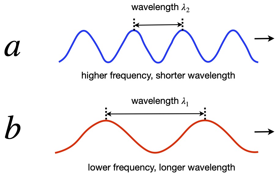
The diagram above shows 2 waves. Recall that the distance between peaks is called the wavelength. The number of wavelengths that cross a point per unit time is called the wave’s frequency. The time it takes to complete one wavelength is the wave’s period. The velocity of the wave is the speed at which the wave moves through space. Some pertinent relationships between these entities are:


where
 is the wave’s frequency
is the wave’s period
is the wave’s wavelength
is the wave’s velocity
Note that waves of short wavelength (figure IV.B.2a) have a high frequency and higher energy while waves of long wavelength (figure IV.B.2b) have a low frequency and lower energy.
Let’s reproduce the setup we had in section IV.B.1.a where we derived gravitational time dilation. We have observer A near a planet of mass and an observer B far enough away from the planet that the gravitational effect from it are negligible i.e., spacetime around be is essentially Minkowski spacetime. All of these objects are floating in empty space and are stationary with respect to each other. Observer A again has a light source. He flashes it twice, at the peaks of the light waves leaving the light source. Thus, the proper time measured by observer A,  , represents the period of the wave. Observer B, again, measures the time interval of the light sent from A as . The equation describing the relationship between and is:
![\[ dt =\frac{d\tau}{ \Biggl( 1 -\frac{2GM}{c^2 r}\Biggr)^{\frac12}} \quad \text{(IV.B.2.1)} \]](https://www.samartigliere.com/wp-content/ql-cache/quicklatex.com-ce764f15f403f14414b8d980516a154c_l3.png "Rendered by QuickLaTeX.com")
From the definitions above, we know that . Therefore:
![\[ f_R = f_E \Biggl( 1 -\frac{2GM}{c^2 r}\Biggr)^{\frac12}} \quad \text{(IV.B.2.2)} \]](https://www.samartigliere.com/wp-content/ql-cache/quicklatex.com-fda7c73cb3144b7c2063a3103081e047_l3.png "Rendered by QuickLaTeX.com")
where
 is the frequency of the light emitted by observer A
 is the frequency of the light received by observer B
Because  is < 1, eq. (IV.B.2.2) tells us that the frequency of light received is lower than when it was emitted, and thus, has less energy. The gravitational field causes it to lose energy just as a particle of matter loses energy as it climbs out of a gravitational field.
This effect was confirmed by a famous experiment performed by Pound and Rebka in 1959. They showed that the frequency of gamma rays emitted at the top of Harvard University’s Jefferson laboratory tower was slightly lower than when they were emitted 74 feet below. Their results have since been replicated multiple times.
IV.B.3 Gravitational Length Contraction
In our discussion of the equivalence principle, we spoke of how, on a rotating disc, an observer at the center of the disc would see measuring rods laid end-to-end on the circumference of the periphery as length contracted. This is because the rods are in motion relative to the observer. And because the rods closer to the the observer are moving will less relative velocity than the rods further away, the degree of length contraction will vary with the radial distance from the observer. We said that, because -per the equivalence principle – acceleration is equivalent to a gravitational effect, we would expect similar length contraction in the presence of a gravitational field, contraction that would increase the closer to the gravitational source we got.
Subsequently, we talked about tidal effects. We noted that, in the presence of gravity, an object will experience elongation in the radial direction and contraction (as in the rotating disc) in the transverse direction.
We can’t directly demonstrate these effects from mathematical manipulation of the Schwarzschild metric. However, some interesting affects can be deduced by examination of this metric as we move in the radial direction toward a massive body.
The first thing we should establish is that the in the Schwarzschild metric equation is not simply the proper distance from the center of a spherically symmetric mass to some point outside the mass. The proper distance between 2 points is the distance we get if we lay out a series of rulers between the 2 points. The problem we have with this in curved spacetime is that the units on the rulers are of different lengths for different points in spacetime. Therefore, to calculate the proper distance along a path in curved spacetime, we have to parameterize the trajectory and take an integral:
![\[ L_0 = \int \| \frac{d}{d\lambda}d\lambda \| \quad \text{(IV.B.3.1)} \]](https://www.samartigliere.com/wp-content/ql-cache/quicklatex.com-75c6e26ac2a80344573ed8a59bbafba5_l3.png "Rendered by QuickLaTeX.com")
where is the path parameter. In this calculation, we assume that and are constant.
 is spacelike (i.e., time is constant). We’re using the mainly minuses metric, thus the expression under the square root sign is negative. So our integral becomes:

Remember that the Schwarzschild metric with constant and is:
 where
where  . This implies that
  . We substitute this value into eq. (IV.B.3.2) and obtain:

So the general equation for proper length between points  in Schwarzschild spacetime is:
![\[ L_0 = \int_a^b dL_0 = \int_{r_1}^{r_2} \sqrt{ \frac{r}{r-R_s}}dr \quad \text{(IV.B.3.4)} \]](https://www.samartigliere.com/wp-content/ql-cache/quicklatex.com-f1925f5ce841dabe22a663424a64c65f_l3.png "Rendered by QuickLaTeX.com")
So in Minkowski (flat) spacetime, where  . Thus, the expression for proper length is simple:
![\[ L_0 = \int_{r_1}^{r_2} 1 \cdot dr = b - a \quad \text{(IV.B.3.5)} \]](https://www.samartigliere.com/wp-content/ql-cache/quicklatex.com-f09431b25a14414ff9094cc8ed9dab36_l3.png "Rendered by QuickLaTeX.com")
But in Schwarzschild spacetime, the relationship is more complicated. Qualitatively, though, we can see that as  ,
,  gets progressively greater than
  . If we want a quantitative evaluation, we need to evaluate the integral in eq. (IV.B.3.4). This is no small task. To see it in all its glory, click .
![\[L_0 = \int \sqrt{ \frac{r}{r-R_s}}dr\]](https://www.samartigliere.com/wp-content/ql-cache/quicklatex.com-39ad4cab8675c646db824d5f960624d8_l3.png "Rendered by QuickLaTeX.com")

![\[ L_0 =\int 2 \frac{z^{2}}{\sqrt{z^{2}-R_{s}}} dz \quad \text{(1)} \]](https://www.samartigliere.com/wp-content/ql-cache/quicklatex.com-ff201e58ce5c010a4d07d475113b8274_l3.png "Rendered by QuickLaTeX.com")


 . That yields:
 . This implies that
  . We put this in for


 , gives us:
![\[L_0 &= R_s \frac12 \sinh(2\theta) + R_s\theta \quad \text{(10)} \]](https://www.samartigliere.com/wp-content/ql-cache/quicklatex.com-bbcf46adccd784b2bbd2d605431625ab_l3.png "Rendered by QuickLaTeX.com")


![\[L_0 &=R_{s} \frac{1}{2} \sinh \left(2\left(\cosh ^{-1} y\right)\right)+R_{s} \cosh ^{-1} y \quad \text{(11)} \]](https://www.samartigliere.com/wp-content/ql-cache/quicklatex.com-29717a51d8e137feee036b7baefad4a1_l3.png "Rendered by QuickLaTeX.com")
 using eq. (9):
 ![\[L_0 &=R_{s} \frac{1}{2} \sinh \left(2 \ln \left(y+\sqrt{y^{2}-1}\right)\right)+R_{s} \ln \left(y+\sqrt{y^{2}-1}\right) \quad \text{(12)} \]](https://www.samartigliere.com/wp-content/ql-cache/quicklatex.com-950b18866c9983d85ae5982401cdcf39_l3.png "Rendered by QuickLaTeX.com")
 :
: 
 of eq.(13):


 in terms of
  (with the caveat that
  and
and  ).
).
 . Thus, for
  :
:![\[ L_{0}=\sqrt{r} \sqrt{r-R_{s}}+R_{s} \ln \left(\sqrt{r}+\sqrt{r-R_{s}}\right) + C \quad \text{(19)} \]](https://www.samartigliere.com/wp-content/ql-cache/quicklatex.com-a5a0c7c7deb4a93caaaf57db3f76a93a_l3.png "Rendered by QuickLaTeX.com")
It turns out that the solution to the indefinite form of the integral in eq. (IV.B.3.4) is:
![\[ L_{0}=\sqrt{r} \sqrt{r}-R_{s}}+R_{s} \ln \left(\sqrt{r}+\sqrt{r-R_{s}}\right) + C \quad \text{(IV.B.3.5)} \]](https://www.samartigliere.com/wp-content/ql-cache/quicklatex.com-646009604ac83966fd6dca72126d2cc4_l3.png "Rendered by QuickLaTeX.com")
If we want to determine the proper distance between 2 points  , we must solve the definite integral:

We can “simplify” eq. (IV.B.3.6) further, as follows:
![\[ L_0 = \sqrt{r_2} \sqrt{r_2-R_{s}} - \sqrt{r_1} \sqrt{r_1-R_{s}} + R_{s} \ln \left(\frac{\sqrt{r_2}+\sqrt{r_2-R_{s}}}{\sqrt{r_1}+\sqrt{r_1-R_{s}}} \right) \quad \text{(IV.B.3.7)} \]](https://www.samartigliere.com/wp-content/ql-cache/quicklatex.com-4f3104cd3594cbada46dfa4832bb3290_l3.png "Rendered by QuickLaTeX.com")
At first glance, eq. (IV.B.3.7) shares elements with – but is not exactly the same as – the equation given by K. Griest, Physics 161: Black Holes: Lecture 9/10: 25/27 Jan (for which he does not supply a derivation):
![\[\Delta \sigma=r_{2} A_{2}-r_{1} A_{1}+\frac{R_{S}}{2} \ln \left(\frac{r_{2} A_{2}+r_{2}-R_{S} / 2}{r_{1} A_{1}+r_{1}-R_{S} / 2}\right) \quad \text{(IV.B.3.8)} \]](https://www.samartigliere.com/wp-content/ql-cache/quicklatex.com-b5e7d9a8db1730e84f02a9974acced73_l3.png "Rendered by QuickLaTeX.com")
where


However, with some algebraic manipulation, we can show that eq. (IV.B.3.7) and eq. (IV.B.3.8) are the same. To see these manipulations, click .
 into eq. (IV.B.3.8), we obtain:
![\[L_0=r_{2} \sqrt{1-\displaystyle \frac{R_s}{r_2}} -r_{1} \sqrt{1-\displaystyle \frac{R_s}{r_1}} +\frac{R_{S}}{2} \ln \left(\frac{r_{2} \sqrt{1-\displaystyle \frac{R_s}{r_2}} +r_{2}-R_{S} / 2}{r_{1} \sqrt{1-\displaystyle \frac{R_s}{r_1}} +r_{1}-R_{S} / 2}\right) \quad \text{(IV.B.3.8a)} \]](https://www.samartigliere.com/wp-content/ql-cache/quicklatex.com-b344ffc6b6bbea542267794cc6439130_l3.png "Rendered by QuickLaTeX.com")

![\[L_0=\sqrt{r_2} \sqrt{r_2 - R_s} -\sqrt{r_1} \sqrt{r_1 - R_s} + \frac{R_{S}}{2} \ln \left(\frac{\sqrt{r_2} \sqrt{r_2 - R_s} +r_{2}-R_{S} / 2}{\sqrt{r_1} \sqrt{r_1 - R_s} +r_{1}-R_{S} / 2}\right) \quad \text{(IV.B.3.8c)} \]](https://www.samartigliere.com/wp-content/ql-cache/quicklatex.com-50ba6f3162e0902bbc534ba0f62bf349_l3.png "Rendered by QuickLaTeX.com")


![\[\ln \frac12 \Bigl(\sqrt{r} + \sqrt{r-R_s}\Bigr)^2 = 2\ln\Bigl(\sqrt{r} + \sqrt{r-R_s}\Bigr) + \ln(\frac12) \quad \text{(IV.B.3.8e)} \]](https://www.samartigliere.com/wp-content/ql-cache/quicklatex.com-349398a98490bbf72ea5fdfa90914b1b_l3.png "Rendered by QuickLaTeX.com")

 , we get:
 is the same as the logarithm term in the formula we derived for
 Griest, in his online book, provides an example of the use of this equation. Consider a black hole with  . If we start at
  and move to
  , we might think that we’ve traveled 10 km. However, if we plug the values above into eq. (IV.B.3.7), we found that the proper distance that we’ve moved is actually 12.51 km. However, if orbit the black hole at
  , we might expect that the circumference of the circle in which we traveled would be
  . However, the circumference that we’d actually measure would be
 . To see why this is so, click .
![\[ds^2 = \Bigl( 1-\displaystyle \frac{R_s}{r} \Bigr)c^2dt^2 - \Bigl( 1-\displaystyle \frac{R_s}{r} \Bigr)^{-1}dr^2 -r^2 d\theta^2 - r^2 \sin^2 \theta d\phi^2 \quad \text{(1)} \]](https://www.samartigliere.com/wp-content/ql-cache/quicklatex.com-74ca421ab01fffee53a8f4f8e7bb922a_l3.png "Rendered by QuickLaTeX.com")
 . Therefore, eq. (1) becomes:

![\[ L_0 &= r \int d\phi \quad \text{(4)} \]](https://www.samartigliere.com/wp-content/ql-cache/quicklatex.com-6e5cfb3e5c3686d27bad723e3bb13f09_l3.png "Rendered by QuickLaTeX.com")

Figure IV.B.3.1, referred to as an embedding diagram, may help to visualize why proper length increases the closer we get to a massive object.
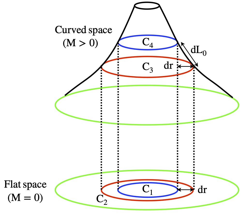
We can see from the diagram that the change in proper distance, , is greater than the change in coordinate distance, , because spacetime is curved.
The paraboloid surface traced out by outer margin of the concentric circles (shown as black half-parabola curves in figure IV.C.1) is referred to as Flamm’s paraboloid. Its formula is:
![\[ w(r) = 2\sqrt(R_s(r-R_s)} \]](https://www.samartigliere.com/wp-content/ql-cache/quicklatex.com-d0abdf5862fa73987bdde746cc9b6076_l3.png "Rendered by QuickLaTeX.com")
where  and
and  are constant and and vary. To see where this formula comes from, click .


IV.B.4 Black Holes
IV.B.4.a Introduction
Notice in the Schwarzschild metric
![\[ g_{\mu \nu} = \begin{bmatrix} 1-\displaystyle \frac{R_s}{r} &0&0&0 \\ 0&-\displaystyle \frac{1}{1-\displaystyle \frac{R_s}{r}}&0&0 \\ 0&0&-r^2&0 \\ &0&0&0&-r^2\sin^2 \theta\end{bmatrix} \quad \text{(IV.B.4.1)} \]](https://www.samartigliere.com/wp-content/ql-cache/quicklatex.com-a9c5b0623d9ed8559e6f039d7a71b57a_l3.png "Rendered by QuickLaTeX.com")
if  , the
, the  portion of the component of the metric goes to infinity. This represents the true singularity that occurs at the center of a black hole, a locus where general relativity no longer defined.
On the other hand, if  the righthand term in the denominator of the
  component of the metric, then the component goes to infinity. However, this is apparent singularity is referred to as a coordinate singularity since we can find coordinates at which this singularity does not occur at this value of . This location (or actually, spherical shell of locations) is called the event horizon of a black hole with center at . The value is called the Schwarzschild radius.
As eigenchris points out in his YouTube video, Relativity 108b: Schwarzschild Metric – Interpretation (Gravitational Time Dilation, Event Horizon), this is similar to what happens at the origin of the polar coordinate system of flat spacetime. At the origin polar coordinates, the value of is always 0 and the variable has an infinite number of values. Thus, the basis vector  is undefined because can’t be negative. And the basis vector
  is undefined because how can we take the derivative of an entity that has more than one value at one time. However, flat spacetime in Cartesian coordinates shows no such problems at the origin.
Coordinate systems have been developed (eg. Eddington-Finkelstein coordinates, Kruskal-Szekeres coordinates) that removes the singularity at .
A black hole occurs when all the mass of an object becomes concentrated to within the object’s Schwarzschild radius. Recall that the Schwarzschild radius of an object is defined as:
![\[ R_s = \displaystyle \frac{2GM}{c^2} \quad \text{(IV.B.4.2)} \]](https://www.samartigliere.com/wp-content/ql-cache/quicklatex.com-1d140acea16c74b1983d970d2163e84f_l3.png "Rendered by QuickLaTeX.com")
where


is very small and is very small. Thus, the Schwarzschild radius of an object is, in general, quite small. For example, the earth’s mass is  . Therefore:

So, to become a black hole, all the mass of the earth would be needed to be compressed to a radius less than 1 cm. Similar calculations show that, to become a black hole, the mass of the sun would need to be compressed down to a radius of less than 2.96 km.
To understand how spacetime is curved around a black hole, let’s look at the behavior of light around one. We do this by looking at light-like geodesics. For a light-like geodesic, tangent vectors have a squared length of zero:
![\[ \| \frac{d}{d\lambda} \|^2 = \frac{dx^{\mu}}{d\lambda} \frac{dx^{\nu}}{d\lambda} g_{\mu \nu}= 0 \quad \text{(IV.B.4.4)} \]](https://www.samartigliere.com/wp-content/ql-cache/quicklatex.com-00b35015f3f3fc249111d52f1838c5cf_l3.png "Rendered by QuickLaTeX.com")
We’ll only consider light beams traveling in the radial direction; and will be kept constant. Therefore, the metric we’ll be working with is reduced to:
![\[ g_{\mu \nu} = \begin{bmatrix} 1-\displaystyle \frac{R_s}{r} &0 \\ 0& -\displaystyle \frac{1}{1-\displaystyle \frac{R_s}{r}} \end{bmatrix} \quad \text{(IV.B.4.5)} \]](https://www.samartigliere.com/wp-content/ql-cache/quicklatex.com-b48ce217a3843d4d55a535cf893cd172_l3.png "Rendered by QuickLaTeX.com")
Eq. (IV.B.4.4) can be re-written:
![\[ \Bigl( \frac{dct}{d\lambda} \Bigr)^2\Bigl( 1-\frac{R_s}{r}\Bigr) - \Bigl( \frac{dr}{d\lambda} \Bigr)^2 \Bigl( \displaystyle \frac{1}{1-\displaystyle \frac{R_s}{r}}\Bigr) = 0 \]](https://www.samartigliere.com/wp-content/ql-cache/quicklatex.com-d8d8e6e1dc8d67946f43bd063aa5cc2c_l3.png "Rendered by QuickLaTeX.com")
![\[ \Bigl( \frac{dct}{d\lambda} \Bigr)^2\Bigl( 1-\frac{R_s}{r}\Bigr) = \Bigl( \frac{dr}{d\lambda} \Bigr)^2 \Bigl( \displaystyle \frac{1}{1-\displaystyle \frac{R_s}{r}}\Bigr) \]](https://www.samartigliere.com/wp-content/ql-cache/quicklatex.com-16349829db49e4156695f74ac3a9c9cb_l3.png "Rendered by QuickLaTeX.com")
![\begin{align*} \Biggl[\Bigl( \frac{dct}{d\lambda} \Bigr)^2\Bigl( 1-\frac{R_s}{r}\Bigr)\Biggr]\Bigl( 1-\frac{R_s}{r}\Bigr) &= \Biggl[\Bigl( \frac{dr}{d\lambda} \Bigr)^2 \Bigl( \displaystyle \frac{1}{1-\displaystyle \frac{R_s}{r}}\Bigr)\Biggr]\Bigl( 1-\frac{R_s}{r}\Bigr) \\ \Bigl( \frac{dct}{d\lambda} \Bigr)^2\Bigl( 1-\frac{R_s}{r}\Bigr)^2 &= \Bigl( \frac{dr}{d\lambda} \Bigr)^2 \\ \pm \frac{dct}{d\lambda}\Bigl( 1-\frac{R_s}{r}\Bigr) &= \frac{dr}{d\lambda} \quad \text{(IV.B.4.6)} \end{align*}](https://www.samartigliere.com/wp-content/ql-cache/quicklatex.com-a4cfc00cdf74e14ad32a334ebc582044_l3.png "Rendered by QuickLaTeX.com")
We can make our parameter anything that we want. Let’s make it  . We get:

What eq. (IV.B.4.7) appears to be saying is that the speed of light varies with position as light beams approach the event horizon of a black hole. However, this is an artifact of coordinate choice. If we measure the speed of light locally (i.e., using proper time and proper length) it will be true in all coordinate systems, and thus, an expression of a physical law, that:
![\[\displaystyle \frac{dL_0}{d\tau} = c \quad \text{(IV.B.4.8)} \]](https://www.samartigliere.com/wp-content/ql-cache/quicklatex.com-90a4b176fd364c8df48ce26d90fa7a24_l3.png "Rendered by QuickLaTeX.com")
Indeed,  is just a ratio of coordinates and coordinates don’t always have physical meaning. In this case, remember:
- is the proper time only for an observer at

- doesn’t measure proper length
As eigenchris notes, the lesson here is: Don’t trust your eyes looking at a graph or coordinates; the only thing we should trust for making physical measurements is the metric.
But let’s take a closer look at eq. (IV.B.4.7). Solving this differential equation gives us:
![\[ct(r) &= \pm \Bigl( r + R_s\ln(r-R_s) \Bigr) + k \quad \text{(IV.B.4.9)} \]](https://www.samartigliere.com/wp-content/ql-cache/quicklatex.com-f2d53294d6664bc5eed9f154fef04f62_l3.png "Rendered by QuickLaTeX.com")
(To see how we got this, click .)

If we plot eq. (IV.B.4.9), with  we get something like figure IV.B.4.1.
The purple graphs are what an observer at infinity would see for light beams heading toward the event horizon of a black hole with a Schwarzschild radius of 2 and varying values of . It’s not easy to see from this diagram, but these curves never reach the horizon. The interpretation of this finding is that the an observer far away from a black hole will see a light beam approach but never reach the horizon.
The red curves represent light beams moving away from the event horizon. Similar to the light beams represented by the red curves, the distant observer never sees the light beams represented by the red curves touch the horizon.
Figure IV.B.4.2, taken from 28:51 of the eigenchris YouTube video, Relativity 108b: Schwarzschild Metric – Interpretation (Gravitational Time Dilation, Event Horizon), shows curves representing light beams inside the horizon (on the left side) as well as those outside the horizon (on the right).
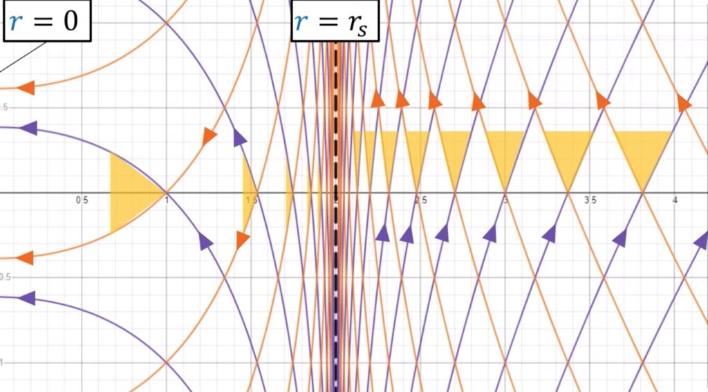
To a distant observer, the light beams outside the horizon never reach the horizon. Furthermore, the light cones nearer the horizon are narrower than those farther away. Those farther away become wider, and at infinity, become normal light cones. Again, this is according to the observer at infinity and, as will be discussed later, is artifact of the coordinates we’re using.
On the other hand, the light beams inside the horizon all point toward the singularity at the center of the black hole and none of them ever touch the horizon. This can be interpreted as meaning that light cannot escape from a black hole, which, in fact, turns out to be true.
IV.B.4.b Alternative Coordinates
IV.B.4.b.i Eddington-Finkelstein
In progress
IV.B.4.b.ii Kruskal-Szekeres
In progress
V Confirmatory Evidence
V.A Mercury Perihelion
As early as the mid nineteenth century, astronomers have known that the orbits of planets around the sun are not perfect ellipses. Instead, each time a planet completes an orbit, the next orbit is slightly “tilted” compared to the previous orbit (figure V.1). This can be made more precise by defining the tilt by the
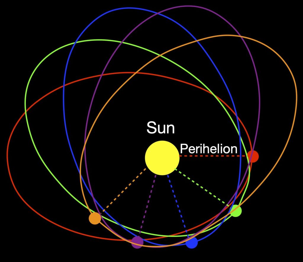
relative position of the planet’s perihelion between successive orbits. As seen in figure V.1, the perihelion is the shortest distance between the sun and the planet during its orbit. Specifically, each time a planet orbits the sun, it doesn’t return to the point from which it started. Instead, it goes a little past that point. The perihelion of the new orbit makes a nonzero angle with the perihelion of the previous orbit. (If that angle were zero, then that would mean the planet returned to its original position.) This is called the advance (or precession of) the perihelion of the planet. It is most pronounced for Mercury, the planet closest to the sun.
The effect is tiny. Mercury, for example, gains an extra angle of only 575 arcseconds each century. There are 3600 arcseconds per degree so that’s a little less than 1/6 of one degree per century(0.1597 of a degree, to be exact; obviously, figure V.1 is not drawn to scale).
Astronomers since the late 1800’s have been able to explain most of this perihelion advance, mainly via the gravitational effect of planets and other objects with mass in the solar system. However, until the advent of general relativity, 43 arcseconds per century of perihelion advance remained unaccounted for. In 1915, Albert Einstein used his theory of general relativity to account for these last 43 arcseconds.
The discussion that follows shows how general relativity solved this problem.
V.A.1 Orbits in Newtonian Gravity
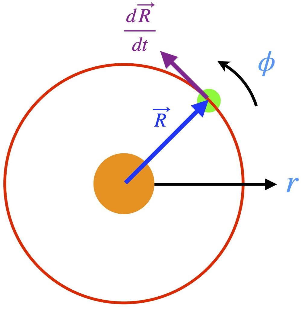
![\[\frac{d\vec{R}}{dr} =\vec{e}_r \quad \frac{d\vec{R}}{d\phi} =\vec{e}_{\phi} \quad \text{(V.A.1)} \]](https://www.samartigliere.com/wp-content/ql-cache/quicklatex.com-5e304ba79ccacd47edc96b15ba8ca00f_l3.png "Rendered by QuickLaTeX.com")
![\[ \frac{d\vec{R}}{dt} = \frac{dr}{dt}\frac{d\vec{R}}{dr} + \frac{d\phi}{dt}\frac{d\vec{R}}{d\phi} \quad \text{(V.A.2)} \]](https://www.samartigliere.com/wp-content/ql-cache/quicklatex.com-53150aad4ad2906d534d92ab4d3af736_l3.png "Rendered by QuickLaTeX.com")
![\[\frac{d\vec{R}}{dt} = \dot{r}\vec{e}_r + \dot{\phi}\vec{e}_{\phi} \quad \text{(V.A.3)} \]](https://www.samartigliere.com/wp-content/ql-cache/quicklatex.com-9ef2fc708fea9e06c107806b78125815_l3.png "Rendered by QuickLaTeX.com")

To see where  comes from, click here.
Now we need to consider angular momentum.

From eq. (V.A.1), if  , then
  . And from eq. (V.A.3), we saw that
  . Substituting these values into eq. (V.A.5), we get:

The magnitude of the cross product  is given by the area of a parallelogram formed from these basis vectors. We know that:
![\[ \vec{e}_r \cdot \vec{e}_r = 1 \quad \Rightarrow \quad \vec{e}_r = 1 \quad \text{(V.A.7)} \]](https://www.samartigliere.com/wp-content/ql-cache/quicklatex.com-bcecc87c78143413848312d1f6d7f6f0_l3.png "Rendered by QuickLaTeX.com")
and
![\[ \vec{e}_{\phi} \cdot \vec{e}_{\phi} =r^2 \quad \Rightarrow \quad \vec{e}_{\phi} = r \quad \text{(V.A.7)} \]](https://www.samartigliere.com/wp-content/ql-cache/quicklatex.com-14bbf95c2978f09584acc00d45de77ed_l3.png "Rendered by QuickLaTeX.com")
Actually,  and
and  but lengths can’t be negative.
Therefore, the parallelogram formed by  and
and  looks like this:
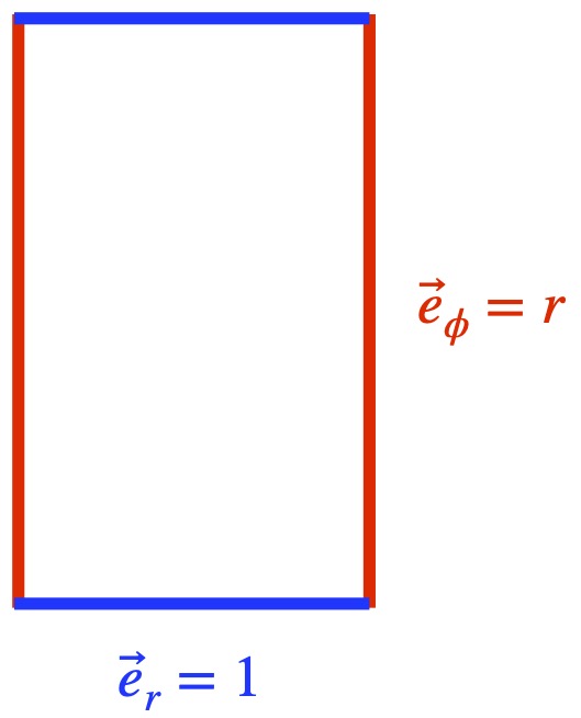
and the area of this parallelogram is  . Recall that the vector associated with the cross product points in a direction perpendicular to plane in which the parallelogram is located; we’ll call it z. The unit basis vector in the z-direction is given by
  . Thus, eq. (V.A.6) becomes:
![\[ \vec{L} = mr\dot{\phi} (r \vec{e}_z) \quad \text{(V.A.8)} \]](https://www.samartigliere.com/wp-content/ql-cache/quicklatex.com-edecac1889bbc84bc24174cb0e48c6db_l3.png "Rendered by QuickLaTeX.com")
This means that the magnitude of the angular momentum is:
![\[ L = mr^2\dot{\phi} \quad \text{(V.A.9)} \]](https://www.samartigliere.com/wp-content/ql-cache/quicklatex.com-fe79560152050bab6fad414a4e0a946e_l3.png "Rendered by QuickLaTeX.com")
Rearranging, we get:
![\[ \dot{\phi} = \frac{L}{mr^2} \quad \text{(V.A.10)} \]](https://www.samartigliere.com/wp-content/ql-cache/quicklatex.com-d3907fb9053fb9031ecf668520b3cb79_l3.png "Rendered by QuickLaTeX.com")
The total energy  of an object – say a planet – orbiting a larger object (like a star) is the planet’s kinetic energy (K.E.) plus its potential energy (P.E):

where
is mass
is the orbiting object’s velocity 
 is the gravitational potential energy
We know from eq. (V.A.4) that:
![\[ v^2 = \Biggl\|\frac{d\vec{R}}{dt}\Biggr\|^2 = \dot{r}^2 + \dot{\phi}^2 r^2 \]](https://www.samartigliere.com/wp-content/ql-cache/quicklatex.com-bedd6cef12d9479a769bcebfc3768629_l3.png "Rendered by QuickLaTeX.com")
and from eq. (V.A.10):
![\[ \dot{\phi} = \frac{L}{mr^2} \]](https://www.samartigliere.com/wp-content/ql-cache/quicklatex.com-414a74b367edab5b9a930c77e075ec67_l3.png "Rendered by QuickLaTeX.com")
Placing these values into eq. (V.A.11) and doing some algebra, we obtain:

From standard Newtonian gravity, the gravitational potential is given by:
![\[ V(r) = -\frac{GM}{r} \quad \text{(V.A.13)} \]](https://www.samartigliere.com/wp-content/ql-cache/quicklatex.com-ed5c5af0360794ddfa7998b7d47dc2f3_l3.png "Rendered by QuickLaTeX.com")
Plugging eq. (V.A.13) into eq. (V.A.12) gives us:

Technically, the  term is related to potential energy and the other terms are related to kinetic energy. However, for this discussion, we group them the way we do in eq. (V.A.14) because the
  term depends on
  and the other terms depend on .
V.A.1 Orbits in General Relativity
We start with the geodesic equation:
![\[ 0 = \frac{d^2 x^{\sigma}}{d\lambda^2} + \Gamma^{\sigma}_{\mu \nu} \frac{dx^{\mu}}{d\lambda} \frac{dx^{\nu}}{d\lambda} \quad \text{(V.A.15)} \]](https://www.samartigliere.com/wp-content/ql-cache/quicklatex.com-6efae568c4d9e4a11a9d2f00b97514ad_l3.png "Rendered by QuickLaTeX.com")
Eq. (V.A.15) actually corresponds to 4 separate equations:
![\[ 0 = \frac{d^2 ct}{d\lambda^2} + \Gamma^{t}_{\mu \nu} \frac{dx^{\mu}}{d\lambda} \frac{dx^{\nu}}{d\lambda} \quad \text{(V.A.16)} \]](https://www.samartigliere.com/wp-content/ql-cache/quicklatex.com-cb2cb2213a7f8868ce1c657a90fffcef_l3.png "Rendered by QuickLaTeX.com")
![\[ 0 = \frac{d^2 r}{d\lambda^2} + \Gamma^{r}_{\mu \nu} \frac{dx^{\mu}}{d\lambda} \frac{dx^{\nu}}{d\lambda} \quad \text{(V.A.17)} \]](https://www.samartigliere.com/wp-content/ql-cache/quicklatex.com-04b45100abe52297c09d6c07305ed2af_l3.png "Rendered by QuickLaTeX.com")
![\[ 0 = \frac{d^2 \theta}{d\lambda^2} + \Gamma^{\theta}_{\mu \nu} \frac{dx^{\mu}}{d\lambda} \frac{dx^{\nu}}{d\lambda} \quad \text{(V.A.18)} \]](https://www.samartigliere.com/wp-content/ql-cache/quicklatex.com-3f66434ecf09c4655f7e9063dd45346d_l3.png "Rendered by QuickLaTeX.com")
![\[ 0 = \frac{d^2 \phi}{d\lambda^2} + \Gamma^{\phi}_{\mu \nu} \frac{dx^{\mu}}{d\lambda} \frac{dx^{\nu}}{d\lambda} \quad \text{(V.A.19)} \]](https://www.samartigliere.com/wp-content/ql-cache/quicklatex.com-5d82a2018f08688329dbe4f54b94da71_l3.png "Rendered by QuickLaTeX.com")
We’re going to assume that  . This is a valid assumption because the mass our object is orbiting is spherically symmetric so we can rotate our coordinate system at any angle and any orbit with will be equivalent. Because is constant, derivatives of are all zero:
![\[\frac{d\theta}{d\lambda} = \frac{d^2\theta}{d^2\lambda} = 0 \quad \text{(V.A.20)} \]](https://www.samartigliere.com/wp-content/ql-cache/quicklatex.com-b9bfd14ed6f829623bc71ebba15cf5e3_l3.png "Rendered by QuickLaTeX.com")
Recall from our derivation of the Schwarzschild metric, we found:
We know that:
is the term in the Schwarzschild metric and equals  . Therefore:
![\[ \partial_r A = 0 - R_s r^{-2}(-1) \]](https://www.samartigliere.com/wp-content/ql-cache/quicklatex.com-cb97f04b5a312fbac1cbd94baf211e32_l3.png "Rendered by QuickLaTeX.com")
![\[ \partial_r A = \frac{R_s}{r^2} \quad \text{(V.A.21)} \]](https://www.samartigliere.com/wp-content/ql-cache/quicklatex.com-db916c4f0da890409ea53296effc960b_l3.png "Rendered by QuickLaTeX.com")
is the absolute value of the  term in the Schwarzschild metric and equals
  . Therefore:

When we insert these values for , and their derivatives into eq. (IV.A.18), we get:

Now that we have values for our Christoffel symbols, we can substitute these into our 4 geodesic equations.
We’ll start with the equation:
![\begin{align*} 0 &= \frac{d^2 ct}{d\lambda^2} + \Gamma^{t}_{\mu \nu} \frac{dx^{\mu}}{d\lambda} \frac{dx^{\nu}}{d\lambda} \\ 0 &= \frac{d^2 ct}{d\lambda^2} + 2\Gamma^{t}_{tr} \frac{dx^{ct}}{d\lambda} \frac{dx^{r}}{d\lambda} \\ 0 &= \frac{d^2 ct}{d\lambda^2} + \Biggl[ 2\frac12 \frac{R_s}{r(r-R_s)} \Biggr] \frac{dx^{ct}}{d\lambda} \frac{dx^{r}}{d\lambda} \\ 0 &= \frac{d^2 ct}{d\lambda^2} + \Biggl[ \frac{R_s}{r(r-R_s)} \Biggr] \frac{dx^{ct}}{d\lambda} \frac{dx^{r}}{d\lambda} \quad \text{(V.A.24)} \end{align*}](https://www.samartigliere.com/wp-content/ql-cache/quicklatex.com-5482e2760234ed80fc1e27768f863007_l3.png "Rendered by QuickLaTeX.com")
Recall from our discussion of Lie derivatives that if the Lie derivative of a vector field is zero, then there is spacetime symmetry (i.e., a conserved quantity) along that vector field. It turns out we can define a conserved quantity from the geodesic equation for . It is:
![\[ \frac{d(ct)}{d\lambda}\Bigl( 1-\frac{R_s}{r} \Bigr) \quad \text{(V.A.25)} \]](https://www.samartigliere.com/wp-content/ql-cache/quicklatex.com-08635d1a16fd0bce465fdd01a1047519_l3.png "Rendered by QuickLaTeX.com")
We can show that this is true, as follows:

So we’ve shown that the derivative of  equals zero which means that is a constant.
We can think of as energy per unit mass:
![\[ \frac{d(ct)}{d\lambda}\Bigl( 1-\frac{R_s}{r} \Bigr) \equiv \frac{E}{m} \equiv \mathcal{E} \quad \text{(V.A.27)} \]](https://www.samartigliere.com/wp-content/ql-cache/quicklatex.com-5085acce3cc30ce6e2d752ccaf55d9d9_l3.png "Rendered by QuickLaTeX.com")
where  is the Schwarzschild spacetime “Energy.”
Note that if we evaluate at  , we get the energy (
 ) term of the 4-momentum:

This justifies our contention that is an energy term.
For the geodesic equation:

We previously listed values for nonzero Christoffel symbols in eq. (V.A.23):

We use these to insert the appropriate values into eq. (V.A.29):

It turns out that we won’t need to use this complicated equation.
For the geodesic equation, there are 3 nonzero Christoffel symbols. In addition, we know that:
![\[ \theta = \frac{\pi}{2} \quad \Rightarrow \quad \frac{d\theta}{d\lambda} = \frac{d^2\theta}{d\lambda^2} = 0 \]](https://www.samartigliere.com/wp-content/ql-cache/quicklatex.com-4e0c88b0f930a08f67199ad83f7ae1fb_l3.png "Rendered by QuickLaTeX.com")
Using these facts, the geodesic equation becomes:

Eq. (V.A.31) shows that setting does not violate our geodesic equations.
For our geodesic equation, we have:

Like the geodesic equation, the geodesic equation is associated with a conserved quantity:  . Here is the proof:
![\begin{align*} &\frac{d}{d\lambda}\Bigl( r^2 \frac{d\phi}{d\lambda} \Bigr) \\ &= \frac{d}{d\lambda}(r^2)\frac{d\phi}{d\lambda} + r^2\frac{d^2\phi}{d\lambda^2} \\ &= 2r\frac{dr}{d\lambda}\frac{d\phi}{d\lambda} + r^2\frac{d^2\phi}{d\lambda^2} \\ &= \Bigl[2r\frac{dr}{d\lambda}\frac{d\phi}{d\lambda} + r^2\frac{d^2\phi}{d\lambda^2}\Bigr]\frac{1}{r^2} \\ &= \underbrace{2\frac{1}{r}\frac{dr}{d\lambda} \frac{d\phi}{d\lambda} + \frac{d^2 \phi}{d\lambda^2}}_{\phi \text{ geodesic equation}} \\ &= 0 \quad \text{(V.A.33)} \end{align*}](https://www.samartigliere.com/wp-content/ql-cache/quicklatex.com-8cc3203a6e65e887ea780cd1af095ce1_l3.png "Rendered by QuickLaTeX.com")
The fact that the derivative of  is zero means that is a constant. The Newtonian angular momentum is given by:
![\[ L = mr^2\frac{d\phi}{d\tau} \quad \text{(V.A.34)} \]](https://www.samartigliere.com/wp-content/ql-cache/quicklatex.com-15106768a768b3454b93882221e1c5a3_l3.png "Rendered by QuickLaTeX.com")
Since we can call our parameter whatever we want, let’s call it . Then:
![\[ L = mr^2\frac{d\phi}{d\lambda} \quad \text{(V.A.35)} \]](https://www.samartigliere.com/wp-content/ql-cache/quicklatex.com-0ceed90c024aaf0359dda987574634ed_l3.png "Rendered by QuickLaTeX.com")
which means:
![\[ r^2\frac{d\phi}{d\lambda} \equiv \frac{L}{m} \equiv \mathcal{L} \quad \text{(V.A.36)} \]](https://www.samartigliere.com/wp-content/ql-cache/quicklatex.com-51cc4021ef90a08edcfec99db587b678_l3.png "Rendered by QuickLaTeX.com")
That is, our conserved quantity represents angular momentum per unit mass. As seen in eq. (V.A.36), we’ll denote this quantity .
So, from our geodesic equations, we’ve derived 2 constants of motion:

and

We need one more piece to come up with an equation that describes the orbit of objects in general relativity: an expression for the length of the tangent vector to our object’s orbit.
We know the squared length of a vector is given by:

Recall that:


Placing the results of eq. (38) and eq. (39) into eq. (37) gives us:
![\begin{align*} \epsilon &= \mathcal{E}^2 \Bigl(\frac{r}{r-R_s} \Bigr)^2 \Bigl( 1-\frac{R_s}{r} \Bigr) - \Bigl( \frac{dr}{d\lambda} \Bigr)^2 \Bigl( 1-\frac{R_s}{r} \Bigr)^{-1} - \Bigl( \frac{\mathcal{L}}{r^2} \Bigr)^2 r^2 \\ \epsilon &= \mathcal{E}^2 \Bigl(\frac{r}{r-R_s} \Bigr)^2 \Bigl( \frac{r-R_s}{r} \Bigr) - \Bigl( \frac{dr}{d\lambda} \Bigr)^2 \Bigl( 1-\frac{R_s}{r} \Bigr)^{-1} - \Bigl( \frac{\mathcal{L}}{r^2} \Bigr)^2 r^2 \\ 0 &= \mathcal{E}^2 \Bigl(\frac{r}{r-R_s} \Bigr) - \Bigl( \frac{dr}{d\lambda} \Bigr)^2 \Bigl( 1-\frac{R_s}{r} \Bigr)^{-1} - \frac{\mathcal{L^2}}{r^2} - \epsilon \\ \Bigl(\frac{r-R_s}{r} \Bigr) \cdot 0 &= \Biggl[\mathcal{E}^2 \Bigl(\frac{r}{r-R_s} \Bigr) - \Bigl( \frac{dr}{d\lambda} \Bigr)^2 \Bigl( 1-\frac{R_s}{r} \Bigr)^{-1} - \frac{\mathcal{L}^2}{r^2} - \epsilon \Biggr] \cdot \Bigl(\frac{r-R_s}{r} \Bigr) \\ 0 &= \mathcal{E}^2 - \Biggl(\frac{dr}{d\lambda} \Biggr)^2 - \Biggl(\frac{r-R_s}{r} \Biggr)\Biggl( \frac{\mathcal{L}^2}{r^2} + \epsilon \Biggr) \\ 0 &= \mathcal{E}^2 - \Biggl(\frac{dr}{d\lambda} \Biggr)^2 - \Biggl( 1-\frac{R_s}{r} \Biggr)\Biggl( \frac{\mathcal{L}^2}{r^2} + \epsilon \Biggr) \\ \mathcal{E}^2 &= \Biggl(\frac{dr}{d\lambda} \Biggr)^2 + \Biggl( 1-\frac{R_s}{r} \Biggr)\Biggl( \frac{\mathcal{L}^2}{r^2} + \epsilon \Biggr) \\ \mathcal{E}^2 &= \Biggl(\frac{dr}{d\lambda} \Biggr)^2 + \frac{\mathcal{L}^2}{r^2} - \frac{R_s \mathcal{L}^2}{r^3} + \epsilon - \epsilon \frac{R_s}{r} \\ \mathcal{E}^2 &= \underbrace{\Biggl(\frac{dr}{d\lambda} \Biggr)^2}_{\text{K.E.}} + \underbrace{\epsilon - \epsilon \frac{R_s}{r} + \frac{\mathcal{L}^2}{r^2} - \frac{R_s \mathcal{L}^2}{r^3}}_{V_{\text{eff}}(r)} \\ \quad \text{(V.A.40)} \end{align*}](https://www.samartigliere.com/wp-content/ql-cache/quicklatex.com-3d66413fb7ff1d3a1d7228c9d284639b_l3.png "Rendered by QuickLaTeX.com")
For light-like geodesics that govern how light beams move,  . For time-like geodesics that govern the motion of massive bodies,
  .
.
We’ll take the case of massive bodies (). For this case, we’ll use and note that:
![\[ \displaystyle R_s = \frac{2GM}{c^2}\]](https://www.samartigliere.com/wp-content/ql-cache/quicklatex.com-6132624ac2fad88bdcf942c9db3a8214_l3.png "Rendered by QuickLaTeX.com")
and
![\[ \epsilon = \frac{d}{d\lambda} \cdot \frac{d}{d\lambda} = \frac{d}{d\tau} \cdot \frac{d}{d\tau} = \vec{U} \cdot \vec{U} = c^2\]](https://www.samartigliere.com/wp-content/ql-cache/quicklatex.com-801c911ebde6c4a82629b04f022caf56_l3.png "Rendered by QuickLaTeX.com")
Substituting these values into eq. (V.A.40), we have:
![\begin{align*} \mathcal{E}^2 &= \Biggl(\frac{dr}{d\lambda} \Biggr)^2 + \epsilon - \epsilon \frac{R_s}{r} + \frac{\mathcal{L}^2}{r^2} - \frac{R_s \mathcal{L}^2}{r^3} \\ \mathcal{E}^2 &= \Biggl(\frac{dr}{d\lambda} \Biggr)^2 + c^2 - \cancel{c^2} \frac{2GM}{\cancel{c^2}}\frac{1}{r} + \frac{\mathcal{L}^2}{r^2} - \frac{2GM}{c^2}\frac{\mathcal{L}^2}{r^3} \\ \frac12 \cdot \mathcal{E}^2 &= \Biggl[\Biggl(\frac{dr}{d\lambda} \Biggr)^2 + c^2 - \frac{2GM}{r} + \frac{\mathcal{L}^2}{r^2} - \frac{2GM}{c^2}\frac{\mathcal{L}^2}{r^3}\Biggr] \cdot \frac12 \\ \frac12 \mathcal{E}^2 &= \frac12\Biggl(\frac{dr}{d\lambda} \Biggr)^2 + \frac12 c^2 - \frac{GM}{r} + \frac{\mathcal{L}^2}{2r^2} - \frac{GM}{c^2}\frac{\mathcal{L}^2}{r^3} \\ & \text{Substituting } \mathcal{L} = \frac{L}{m} \text{ and } \mathcal{E} = \frac{E}{m} \text{ gives us:} \\ \Biggl[\frac12 \Bigl(\frac{E}{m}\Bigr)^2 &= \frac12\Biggl(\frac{dr}{d\lambda} \Biggr)^2 + \frac12 c^2 - \frac{GM}{r} + \frac{L^2}{2m^2r^2} - \frac{GM}{c^2}\frac{L^2}{m^2r^3}\Biggr] \cdot m \\ \frac12 \Bigl(\frac{E}{m}\Bigr)^2 m &= \frac12 m \Biggl(\frac{dr}{d\lambda} \Biggr)^2 + \frac12 mc^2 - m\Biggl(\frac{GM}{r} + \frac{L^2}{2m^2r^2} - \frac{GM}{c^2}\frac{L^2}{m^2r^3}\Biggr) \\ \frac12 \Biggl(\frac{E^2}{m} - mc^2\Biggr) &= \frac12 m \Biggl(\frac{dr}{d\lambda} \Biggr)^2 - m\Biggl(\frac{GM}{r} + \frac{L^2}{2m^2r^2} - \frac{GM}{c^2}\frac{L^2}{m^2r^3}\Biggr) \\ \quad \text{(V.A.41)} \end{align*}](https://www.samartigliere.com/wp-content/ql-cache/quicklatex.com-9bd62c3d112cf0e28415b96e939ce0ad_l3.png "Rendered by QuickLaTeX.com")
We can also arrive at this equation by using action principle. To see this, click .
![\[ \delta A=\delta \int -mcds \quad \text{(1)} \]](https://www.samartigliere.com/wp-content/ql-cache/quicklatex.com-a23e8cce5de2e0811f28ea86a1211a6e_l3.png "Rendered by QuickLaTeX.com")
![\[ ds^{2}=c^{2}dt^{2}=g_{\mu \nu }dx^{u}dx^{\nu } \quad \text{(2)} \]](https://www.samartigliere.com/wp-content/ql-cache/quicklatex.com-bfa1ba0763c0106819c8bac359d768d7_l3.png "Rendered by QuickLaTeX.com")
![\[ ds^{2}=\left( 1-\dfrac{2GM}{c^{2}r}\right) c^{2}dt^{2}-\left( \dfrac{1}{1-\dfrac{2GM}{c^{2}r}}\right) dr^{2}-r^{2}d\theta ^{2}-r^{2}\sin ^{2}\theta d\phi ^{2} \quad \text{(3)} \]](https://www.samartigliere.com/wp-content/ql-cache/quicklatex.com-d42b78234047af4112c0e599221c2992_l3.png "Rendered by QuickLaTeX.com")
![\[\theta =\dfrac{\pi }{2}\quad \Rightarrow \sin \theta =1 \quad \text{(4)} \]](https://www.samartigliere.com/wp-content/ql-cache/quicklatex.com-e5243417c29daca29d8e74e5e935956b_l3.png "Rendered by QuickLaTeX.com")
 ),
),  . Finally, we recall from special relativity that, when we use the mostly minuses form of the metric,
![\[ds^{2}&=\left( 1-\dfrac{2GM}{c^{2}r}\right) c^{2}dt^{2}-\left( \dfrac{1}{1-\dfrac{2GM}{c^{2}r}}\right) dr^{2}-r^{2} d\phi ^{2} = c^2d\tau^2 \quad \text{(5)} \]](https://www.samartigliere.com/wp-content/ql-cache/quicklatex.com-37affed9d7110908dc32ade03c1f29ec_l3.png "Rendered by QuickLaTeX.com")
![\[ ds}&=\sqrt{\left( 1-\dfrac{2GM}{c^{2}r}\right) c^{2}dt^{2}-\left( \dfrac{1}{1-\dfrac{2GM}{c^{2}r}}\right) dr^{2}-r^{2} d\phi ^{2}} = c^2d\tau^2 \quad \text{(6)} \]](https://www.samartigliere.com/wp-content/ql-cache/quicklatex.com-1eb17679a1fc5429dd7ab6f74eb4c784_l3.png "Rendered by QuickLaTeX.com")
![\[A=\int -mc\underbrace{\sqrt{\left( 1-\dfrac{2GM}{c^{2}r}\right) c^{2}d\tau ^{2}-\dfrac{1}{1-\dfrac{2GM}{c^{2}r}}dr^{2}-r^{2}d\phi ^2}}_{c}\,d\tau \quad \text{(7)} \]](https://www.samartigliere.com/wp-content/ql-cache/quicklatex.com-8a3744b847d2ee09d0e74a31d55a79f9_l3.png "Rendered by QuickLaTeX.com")
 . Therefore, the expression involving the square root in eq. (7) equals
 ![\[\mathcal{L} = -mc^2 \quad \text{(8)} \]](https://www.samartigliere.com/wp-content/ql-cache/quicklatex.com-96d6fd28b36f2e55dc3b63d29baa4c19_l3.png "Rendered by QuickLaTeX.com")
 . Then:
 ![\[A=\int -mc\underbrace{\sqrt{\left( 1-\dfrac{2GM}{c^{2}r}\right) c^{2}\dot{t} ^{2}-\dfrac{1}{1-\dfrac{2GM}{c^{2}r}}d\dot{r}^{2}-r^{2}d\dot{\phi} ^2}}_{c}\,d\tau \quad \text{(9)} \]](https://www.samartigliere.com/wp-content/ql-cache/quicklatex.com-d06bb3195602a0a2c7ff10f15de2d388_l3.png "Rendered by QuickLaTeX.com")
 (since there are no “t” terms in our Lagrangian. This implies:
![\[ \frac{d}{d\tau}\frac{\partial \mathcal{L}}{\partial \dot{t}} = \frac{d}{\cancel{d\tau}}\left(\frac{\partial \mathcal{L}}{\partial \frac{dt}{\cancel{d\tau}}}\right) = \frac{\partial \mathcal{L}}{dt} = 0 \, \Rightarrow \, \frac{d}{d\tau}\frac{\partial \mathcal{L}}{\partial \dot{t}} = \text{ constant} \quad \text{(10)} \]](https://www.samartigliere.com/wp-content/ql-cache/quicklatex.com-50f1d2e76d876787e09e9e638f1dfd1d_l3.png "Rendered by QuickLaTeX.com")
![\[\dfrac{\partial L}{\partial \dot {t}}=\dfrac{-mc\left( 1-\dfrac{2GM}{c^{2}r}\right) c^2 \dot {t}}{c}=-mc^{2}\left( 1-\dfrac{2GM}{c^{2}r}\right) \dot{t }=-E \quad \text{(11)} \]](https://www.samartigliere.com/wp-content/ql-cache/quicklatex.com-d9b516d7adb78f34220bad85e186bb12_l3.png "Rendered by QuickLaTeX.com")
![\[ \dot{t} = \frac{E}{mc^2\left(1-\displaystyle}\frac{2GM}{c^2 r}\right)} \quad \text{(12)} \]](https://www.samartigliere.com/wp-content/ql-cache/quicklatex.com-39cb1788f35ccccac9762e80bde2422d_l3.png "Rendered by QuickLaTeX.com")
 . Perhaps the 2 is absorbed into the constant
  .
.![\[\dfrac{\partial L}{\partial \phi }=0\Rightarrow \dfrac{\partial L}{\partial \dot{\phi} }=\text{const} \quad \text{(13)} \]](https://www.samartigliere.com/wp-content/ql-cache/quicklatex.com-437440829eb3c2af9146fa1cc7995021_l3.png "Rendered by QuickLaTeX.com")
![\[ \dfrac{\partial \mathcal{L}}{\partial \dot{\phi} }=-mc\dfrac{r^{2}\dot{\phi }}{c}=mr^2\dot{\phi}=L \quad \text{(14)} \]](https://www.samartigliere.com/wp-content/ql-cache/quicklatex.com-a6c056d56a58e468dba8ef20080fc6a4_l3.png "Rendered by QuickLaTeX.com")
![\[ \omega_{\phi }=\dot{\phi}= \dfrac{L}{mr^2} \quad \text{(15)} \]](https://www.samartigliere.com/wp-content/ql-cache/quicklatex.com-945bad3378466b377e793f028b4ca426_l3.png "Rendered by QuickLaTeX.com")
 . This implies that
  . Plugging in values from our Lagrangian, we have:
![\[ m^{2}c^{2}\left[ \dfrac{E^{2}}{m^{2}c^{2}\left( 1-\dfrac{2Gm}{c^{2}r}\right) }-\dfrac{\dot{r}^{2}}{1-\dfrac{2GM}{c^{2}r}}-\dfrac{L^{2}}{m^{2}r^{2}}\right] =m^{2}c^{4} \quad \text{(16)} \]](https://www.samartigliere.com/wp-content/ql-cache/quicklatex.com-6f9e72ce60b387ed81381bf258000e12_l3.png "Rendered by QuickLaTeX.com")
![\[ \frac{E^{2} m c^{2}}{m^{2} c^{2}\left(1-\frac{2 G M}{c^{2} r}\right)}-m^{2} c^{4}=\frac{\dot{r}^{2} m^{2} c^{2}}{1-\frac{2 G M}{c^{2} r}}+\frac{L^{2} m^{2} c^{2}}{m^{2} r^{2}} \]](https://www.samartigliere.com/wp-content/ql-cache/quicklatex.com-834a4658c5f8afa65ff5044946574f78_l3.png "Rendered by QuickLaTeX.com")
![\[ E^{2}-m^{2} c^{4}\left(1-\frac{2 G M}{c^{2} r}\right)=\dot{r}^{2} m^{2} c^{2}+\left(\frac{L^{2} m^{2} c^{2}}{m^{2} r^{2}}\right)\left(1-\frac{2 G M}{c^{2} r}\right) \]](https://www.samartigliere.com/wp-content/ql-cache/quicklatex.com-95ba39e5210640c1006feb62b7a405bf_l3.png "Rendered by QuickLaTeX.com")
![\[ E^{2}-m^{2} c^{4}+\frac{m^{2} c^{4} 2 G M}{c^{2} r}=\dot{r}^{2} m^{2} c^{2}+\frac{L^{2} m c^{2}}{m^{2} r^{2}}-\frac{L^{2} m^{2} c^{2} 2 G M}{m^{2} r^{2} c^{2} r} \]](https://www.samartigliere.com/wp-content/ql-cache/quicklatex.com-b25fd7851a44d07bbc65c70f6f33b323_l3.png "Rendered by QuickLaTeX.com")
![\[ E^{2}-m^{2} c^{4}=-\frac{m^{2} c^{2} 2 G M}{r}+\dot{r}^{2} m^{2} c^{2}+\frac{L^{2} c^{2}}{m r^{2}}-\frac{L^{2} 2 G M}{r^{3}} \]](https://www.samartigliere.com/wp-content/ql-cache/quicklatex.com-55d9f71d91463c2c226c62580d935cef_l3.png "Rendered by QuickLaTeX.com")
![\[ \frac{E^{2}-m^{2} c^{4}}{m c^{2}}=\frac{2 m G M}{r}+m \dot{r}^{2}+\frac{L^{2}}{m^{2} r^{2}}-\frac{L^{2} 2 G M}{m^{2} c^{2} r^{3}} \]](https://www.samartigliere.com/wp-content/ql-cache/quicklatex.com-278ec5e02ecb274a79957f37423acdad_l3.png "Rendered by QuickLaTeX.com")
![\[ \frac{1}{2} \frac{E^{2}-m^{2} c^{4}}{m c^{2}}=\frac{m G M}{r}+\frac{1}{2} m \dot{r}^{2}+\frac{1}{2} \frac{L^{2}}{m r^{2}}-\frac{L^{2} G m}{m c^{2} r^{3}} \quad \text{(17)} \]](https://www.samartigliere.com/wp-content/ql-cache/quicklatex.com-fc51a50b4456f6babdfa0ec960ab3eeb_l3.png "Rendered by QuickLaTeX.com")
![\[ \underbrace{\frac{1}{2} \frac{E^{2}-m^{2} c^{4}}{m c^{2}}}_{\text{Total Energy}}=\underbrace{\frac{1}{2} m \dot{r}^{2}}_{\text{Kinetic Energy}}+\quad\underbrace{\frac{m G M}{r}+\frac{1}{2} \frac{L^{2}}{m r^{2}}-\frac{L^{2} G m}{m c^{2} r^{3}}}_{\text{Potential Energy}} \quad \text{(18)} \]](https://www.samartigliere.com/wp-content/ql-cache/quicklatex.com-2fd9dc078130c270e7b578f3ab7be6cb_l3.png "Rendered by QuickLaTeX.com")
![\[ (E-V)^{2}=p c^{2}+m^{2} c^{4} \]](https://www.samartigliere.com/wp-content/ql-cache/quicklatex.com-076f4d471f66a42fc503e3e9b46cda9d_l3.png "Rendered by QuickLaTeX.com")
![\[ E^{2}+V^{2}-2 E V=p c^{2}+m^{2} c^{4} \]](https://www.samartigliere.com/wp-content/ql-cache/quicklatex.com-4db308cdbe35f270c5904ae027d1a992_l3.png "Rendered by QuickLaTeX.com")
![\[ E^{2}-m^{2} c^{4}=p c^{2}-V^{2}+2 E V \]](https://www.samartigliere.com/wp-content/ql-cache/quicklatex.com-c53bcbe55b1a01d9e5cf6b0293c84a1a_l3.png "Rendered by QuickLaTeX.com")
![\[ \frac{1}{2} \frac{E^{2}-m^{2} c^{4}}{m c^{2}}=\frac{p^{2} c^{2}}{2 m c^{2}}-\frac{V^{2}}{2 m c^{2}}+\frac{2 E V}{2 m c^{2}} \]](https://www.samartigliere.com/wp-content/ql-cache/quicklatex.com-e42090b906ec02b27db4e7f09682b01c_l3.png "Rendered by QuickLaTeX.com")
![\[ \frac{1}{2} \frac{E^{2}-m^{2} c^{4}}{m c^{2}}=\frac{p^{2}}{2 m}-\frac{V^{2}}{2 m c^{2}}+\frac{E V}{m c^{2}} \quad \text{(19)} \]](https://www.samartigliere.com/wp-content/ql-cache/quicklatex.com-75d1436e49bdd6c17850e0af21e12941_l3.png "Rendered by QuickLaTeX.com")
 . This gives us:
![\[ \frac{1}{2} \frac{E^{2}-m^{2} c^{4}}{m c^{2}}=\frac{p^{2}}{2 m}+\frac{E V}{m c^{2}} \quad \text{(20)} \]](https://www.samartigliere.com/wp-content/ql-cache/quicklatex.com-bb21ae8063c5f7e03646ac501f222205_l3.png "Rendered by QuickLaTeX.com")
 . Thus:
 represents total energy in nonrelativistic physics.
![\[ \underbrace{\frac{1}{2}\frac{E^2}{m} - mc^2}_{\text{eigenchris}} \quad \text{vs} \quad \underbrace{\frac{1}{2}\frac{E^{2}-m^{2}c^{4}}{mc^{2}}}_{\text{Pesaresi}} \]](https://www.samartigliere.com/wp-content/ql-cache/quicklatex.com-da648eab9489a2212e667c566a4bef80_l3.png "Rendered by QuickLaTeX.com")
![\[ \frac{1}{2}\frac{E^2}{m}\frac{c^2}{c^2} - mc^2\frac{mc^2}{mc^2}} = \frac{1}{2}\frac{E^{2}c^2-m^{2}c^{4}}{mc^{2}} \quad \text{(22)} \]](https://www.samartigliere.com/wp-content/ql-cache/quicklatex.com-1960484603aae16477820971e511f0ef_l3.png "Rendered by QuickLaTeX.com")
 term. I haven’t seen a derivation of this term from other sources although, I admit, my search has been far from exhaustive.
To summarize:
Newtonian Orbits:
![\[ \underbrace{E}_{E_{\text{tot}}} = \underbrace{\frac12 m\Bigl( \frac{dr}{dt} \Bigr) ^2}_{\text{K.E.}}+ \underbrace{m\Bigl( -\frac{GM}{r} + \frac{L^2}{2m^2r^2} \Bigr) }_{V_{\text{eff}}(r)} \quad \text{(V.A.40)} \]](https://www.samartigliere.com/wp-content/ql-cache/quicklatex.com-3e4c94fbb485de69440bc9894525418b_l3.png "Rendered by QuickLaTeX.com")
General Relativity Orbits:
![\[ \underbrace{\frac12\Bigl(\frac{E^2}{m} - mc^2 \Bigr)}_{E_\text{tot}}} = \underbrace{\frac12 \Bigl( \frac{dr}{dt} \Bigr)^2}_{\text{K.E.}} + \underbrace{m\Bigl( -\frac{GM}{r} + \frac{L^2}{2m^2r^2} - \frac{GM}{c^2}\frac{L^2}{m^2r^3} \Bigr)}_{V_{\text{eff}}(r)} \quad \text{(V.A.41)} \]](https://www.samartigliere.com/wp-content/ql-cache/quicklatex.com-faadf72385e801cd9d3525f0a8df219a_l3.png "Rendered by QuickLaTeX.com")
V.A.3 Derivations
Our task, ultimately, is to derive to equations of motion of the planet Mercury around the sun. At the time of Einstein’s original paper on the subject, Schwarzschild had not yet come up with his solution to Einstein’s field equation. Therefore, Einstein estimated the advance of the perihelion of Mercury using perturbation theory. I, personally, find Einstein’s original paper difficult to follow. In addition, once the Schwarzschild metric became known, it afforded more accurate calculation of Mercury’s perihelion advance. For these reasons, I won’t discuss Einstein’s solution, but rather, will present a well-known solution that uses the equations we’ve already derived. I’ll also present a second derivation that I believe is easier to follow. Because the derivations are mathematically tedious, I’ll just provide the result in the main text, then plug in some numbers to show that general relativity, indeed, accounts for the unexplained portion of Mercury’s perihelion precession. For those interested in actually seeing the derivations, click on the following link:
![\[ \mathcal{E}^2 = \Biggl(\frac{dr}{d\lambda} \Biggr)^2 + \epsilon - \epsilon \frac{R_s}{r} + \frac{\mathcal{L}^2}{r^2} - \frac{R_s \mathcal{L}^2}{r^3} \quad \text{(1)} \]](https://www.samartigliere.com/wp-content/ql-cache/quicklatex.com-86e2aa4c920ecdf2f265fdf07e6bcd7c_l3.png "Rendered by QuickLaTeX.com")
 and
and ![\[ \mathcal{E}^2 = \Biggl(\frac{dr}{d\tau} \Biggr)^2 + c^2 - c^2 \frac{R_s}{r} + \frac{\mathcal{L}^2}{r^2} - \frac{R_s \mathcal{L}^2}{r^3} \quad \text{(2)} \]](https://www.samartigliere.com/wp-content/ql-cache/quicklatex.com-6c7e4f49462cb66548d9cef87825dd56_l3.png "Rendered by QuickLaTeX.com")
 as:
as:![\[ \frac{dr}{d\tau} = \frac{dr}{d\phi}\frac{d\phi}{d\tau} \quad \text{(3)} \]](https://www.samartigliere.com/wp-content/ql-cache/quicklatex.com-e2f7b35415a9052de537dbe21c8b04e1_l3.png "Rendered by QuickLaTeX.com")
 . Substituting this into eq. (2), we get:
 . This gives us:
![\[ (\mathcal{E}^2 - c^2) \frac{r^2}{\mathcal{L}^2} = \Biggl(\frac{dr}{d\phi}\Biggr)^2\frac{1}{r^2} - c^2\frac{R_s r}{\mathcal{L}^2} + 1 - \frac{R_s}{r} \quad \text{(5)} \]](https://www.samartigliere.com/wp-content/ql-cache/quicklatex.com-1ff6a623efb87e8dbebef077961739c2_l3.png "Rendered by QuickLaTeX.com")
 . This allows us to do the following:
![\[ (\mathcal{E}^2 - c^2) \frac{1}{\mathcal{L}^2}\frac{1}{u^2} = \Biggl(\frac{du}{d\phi}\Biggr)^2\frac{1}{u^2} - c^2\frac{R_s}{\mathcal{L}^2}\frac{1}{u} + 1 - R_s u \quad \text{(7)} \]](https://www.samartigliere.com/wp-content/ql-cache/quicklatex.com-16f8223bf8e78a759df1481bb0e5afac_l3.png "Rendered by QuickLaTeX.com")
 yields:
![\[ (\mathcal{E}^2 - c^2) \frac{1}{\mathcal{L}^2} = \Biggl(\frac{du}{d\phi}\Biggr)^2 - \frac{c^2 R_s}{\mathcal{L}^2}u + u^2 - R_s u^3 \quad \text{(8)} \]](https://www.samartigliere.com/wp-content/ql-cache/quicklatex.com-aec4ade78fc1ddb069d33437354ef630_l3.png "Rendered by QuickLaTeX.com")
 generating this equation:
![\[ 0 = 2\Biggl(\frac{du}{d\phi}\Biggr)\frac{d^2u}{d\phi^2} - \frac{c^2 R_s}{\mathcal{L}^2}\frac{du}{d\phi} + 2u\frac{du}{d\phi} - 3R_s u^2 \frac{du}{d\phi} \quad \text{(9)} \]](https://www.samartigliere.com/wp-content/ql-cache/quicklatex.com-456f9701838cbc5c418db68d548713a2_l3.png "Rendered by QuickLaTeX.com")
 . We obtain:
![\[ 0 = 2\frac{d^2u}{d\phi^2} - \frac{c^2 R_s}{\mathcal{L}^2} + 2u - 3R_s u^2 \quad \text{(10)} \]](https://www.samartigliere.com/wp-content/ql-cache/quicklatex.com-9a946c0b2362bcb8268ddabcf4203e94_l3.png "Rendered by QuickLaTeX.com")
 gives:
 . We get:
 and insert it into eq. (12). We get:
![\[0 = \frac{d^2w}{d\phi^2} -1 + w - \alpha w^2 \quad \quad \text{(13)} \]](https://www.samartigliere.com/wp-content/ql-cache/quicklatex.com-92d4dc1b3f982ba89c59e1d14868471e_l3.png "Rendered by QuickLaTeX.com")
![\[\underbrace{\frac{d^2w}{d\phi^2} + w}_{\substack{\text{Simple Harmonic}\\ \text{Oscillator}}} = \underbrace{1}_{\substack{\text{Newtonian}\\ \text{Orbits}}} + \underbrace{\alpha w^2}_{\substack{\text{G.R.}\\ \text{Correction}}} \quad \quad \text{(14)} \]](https://www.samartigliere.com/wp-content/ql-cache/quicklatex.com-e603d6a3b216fa58dafd26e04804c8b7_l3.png "Rendered by QuickLaTeX.com")
 is just the equation for the harmonic oscillator. Its solution is
  .
. is the equation for an ellipse. Its solution is
  where
where  is the eccentricity of the ellipse. To see how we arrive at this result, click .
 where
where is the homogeneous equation (in this context, referred to as the complimentary equation)
 is called the particular solution, the solution to the equation
 ![\[ w^{\prime \prime} + w = 0 \quad \text{(14.1)} \]](https://www.samartigliere.com/wp-content/ql-cache/quicklatex.com-5a9e7189fe54a30fa7665493e6d51107_l3.png "Rendered by QuickLaTeX.com")
 . So
. So![\[ w^{\prime \prime}e^{rt} + e^{rt} = 0 \quad \text{(14.2)} \]](https://www.samartigliere.com/wp-content/ql-cache/quicklatex.com-906b3967b510600acf20134490885b9e_l3.png "Rendered by QuickLaTeX.com")
![\[ r^2e^{rt} + e^{rt} = 0 \quad \text{(14.3)} \]](https://www.samartigliere.com/wp-content/ql-cache/quicklatex.com-54abf4f948b5cdad9e632ef424ffb6cc_l3.png "Rendered by QuickLaTeX.com")
![\[ e^{rt}(r^2 + 1) = 0 \quad \text{(14.4)} \]](https://www.samartigliere.com/wp-content/ql-cache/quicklatex.com-294ba0f9e0223b6efbfa34e957b31e5c_l3.png "Rendered by QuickLaTeX.com")
![\[ r^2 + 1 = 0 \, \Rightarrow \, r=\pm i \, \Rightarrow \, w = e^{i\phi} \text{ and } w = e^{-i\phi} \quad \text{(14.5)} \]](https://www.samartigliere.com/wp-content/ql-cache/quicklatex.com-2f327e4b7133f8ce247b81bef6eb54ad_l3.png "Rendered by QuickLaTeX.com")
![\[ w = C_3 e^{i\phi} + C_4 e^{-i\phi} \quad \text{(14.6)} \]](https://www.samartigliere.com/wp-content/ql-cache/quicklatex.com-9ae38f7c43a665ba67f08c74d4cbec6a_l3.png "Rendered by QuickLaTeX.com")
 and
and are constants. In the case that we’ll be working with, we’ll usually want to have real solutions to our equations. We can use Euler’s relationship to convert eq. (14.6) to real solutions as follows:
![\[ e^{i\phi} = \cos \phi + i\sin \phi \]](https://www.samartigliere.com/wp-content/ql-cache/quicklatex.com-bf56ec2990d1db23b5069f8426cea6cb_l3.png "Rendered by QuickLaTeX.com")
![\[ e^{-i\phi} = \cos (-\phi) + i\sin -(\phi) = \cos \phi - i\sin \phi \]](https://www.samartigliere.com/wp-content/ql-cache/quicklatex.com-5d51aa52cb5da0e83ed3f2b4af8f3268_l3.png "Rendered by QuickLaTeX.com")

 , then
  .
. , then
  .
.![\[ w = C_1 \cos\phi + C_2 \sin\phi \quad \text{(14.8)} \]](https://www.samartigliere.com/wp-content/ql-cache/quicklatex.com-2b0c37b73a524f93f7ce2c529dd11757_l3.png "Rendered by QuickLaTeX.com")
 , eq. (14.8) becomes
  which is the equation of the harmonic oscillator.
![\[ w^{\prime \prime} + w = 1 \quad \text{(14.9)} \]](https://www.samartigliere.com/wp-content/ql-cache/quicklatex.com-cb6ab8beace3aa48dfb8202465775217_l3.png "Rendered by QuickLaTeX.com")
 . Then
  and
and  . We plug these values into the eq. (14.9) and get
  .
. . Thus:
![\[ w = w_0 + w_p = C_1 \cos \phi + C_2 \sin \phi + 1 \quad \text{(14.10)} \]](https://www.samartigliere.com/wp-content/ql-cache/quicklatex.com-bbdf0845f839f162d1e87bad0228fd5e_l3.png "Rendered by QuickLaTeX.com")
![\[ w = 1 + C_1 \cos \phi \quad \text{(14.11)} \]](https://www.samartigliere.com/wp-content/ql-cache/quicklatex.com-80a8ca5d39f8fe47a698aa6a2c8041fc_l3.png "Rendered by QuickLaTeX.com")
 but
but  in eq. (14.11) is proportional to
  . The meaning of this equation is that the distance between the focal point of the ellipse (in our case, the source of gravity like the sun) and the ellipse margin (i.e., the path of an orbiting body) varies periodically.
![\[ w = w_0 + \alpha w_1 + \alpha^2 w_2 + \dots \]](https://www.samartigliere.com/wp-content/ql-cache/quicklatex.com-c7ea08f8e537e4c925f621d699a15c38_l3.png "Rendered by QuickLaTeX.com")
![\[ \frac{d^2}{d\phi^2}(w_0 + \alpha w_1 + \dots) + (w_0 + \alpha w_1 + \dots) = 1 + \alpha(w_0 + \alpha w_1 + \dots)^2 \quad \text{(15)} \]](https://www.samartigliere.com/wp-content/ql-cache/quicklatex.com-486cba185bef5f46e14c217fab0b06df_l3.png "Rendered by QuickLaTeX.com")
![\[ \left(\frac{d^2w_0}{d\phi^2} + w_0\right) + \alpha\left( \frac{d^2w_1}{d\phi^2} + w_1 \right) + \dots = 1 + \alpha(w_0 + \alpha w_1 + \dots)^2 \quad \text{(16)} \]](https://www.samartigliere.com/wp-content/ql-cache/quicklatex.com-36833d8a4a3352f070b784cf59c7f919_l3.png "Rendered by QuickLaTeX.com")
 and higher since
  . We obtain:
![\[ \frac{d^2w_0}{d\phi^2} + w_0 = \alpha(w_0 + \alpha w_1 + \dots)^2 \quad \text{where} \,\, w_0(\phi) = 1 + e\cos \phi \quad \text{(17)} \]](https://www.samartigliere.com/wp-content/ql-cache/quicklatex.com-38129d120ffa60f6d237a1d94cc5b1b2_l3.png "Rendered by QuickLaTeX.com")
![\[ \cancel{\alpha}\left(\frac{d^2w_1}{d\phi^2} + w_1\right) = \cancel{\alpha} w_0^2 = \cancel{\alpha}\left(1 + e\cos \phi\right)^2 \]](https://www.samartigliere.com/wp-content/ql-cache/quicklatex.com-ec1f9c1ed94ca8338d68948efdbf1c4b_l3.png "Rendered by QuickLaTeX.com")
![\[ \frac{d^2w_1}{d\phi^2} + w_1 = w_0^2 = \left(1 + e\cos \phi\right)^2 \quad \text{(18)} \]](https://www.samartigliere.com/wp-content/ql-cache/quicklatex.com-a72cee43b74a341964d545e4c2a36b21_l3.png "Rendered by QuickLaTeX.com")
![\[ \frac{d^2w_1}{d\phi^2} + w_1 = 1 + 2e\cos\phi + e^2\cos^2\phi \quad \text{(19)} \]](https://www.samartigliere.com/wp-content/ql-cache/quicklatex.com-064d769c3182aafb8dbf7370496a3270_l3.png "Rendered by QuickLaTeX.com")
 to replace the
  term in eq. (19). That gives us:
![\[\frac{d^2w_1}{d\phi^2} + w_1 &= \left(1 + \frac12 e^2\right) + 2e\cos\phi + \frac12 e^2 \cos2\phi \quad \text{(20)} \]](https://www.samartigliere.com/wp-content/ql-cache/quicklatex.com-9bd6401106ca1fcead720a3ce76fb509_l3.png "Rendered by QuickLaTeX.com")
![\[ w^{\prime\prim} + w = 1 + \frac12 e^2 \quad \text{(20.1)} \]](https://www.samartigliere.com/wp-content/ql-cache/quicklatex.com-368a379bcf69b5f85794e9116312db47_l3.png "Rendered by QuickLaTeX.com")
 and
and  . Plugging these back into our initial equation, we have:
![\[ w{\prime \prime} + w = 2e\cos\phi \quad \text{(20.3)} \]](https://www.samartigliere.com/wp-content/ql-cache/quicklatex.com-36e95dc2666dab56e4e3f207bab27bcf_l3.png "Rendered by QuickLaTeX.com")
 . However, because
  and
and  are contained in the complementary solution, if we use this, terms will cancel and we’ll get zero. Thus, we have to put a
 ![\[ w_p = \phi A\sin\phi + \phi B\cos\phi \quad \text{(20.4)} \]](https://www.samartigliere.com/wp-content/ql-cache/quicklatex.com-e770732bc725f1225426d123904c435d_l3.png "Rendered by QuickLaTeX.com")


![\[ 2A\cos\phi - 2B\sin\phi = 2e \cos\phi \quad \text{(20.8)} \]](https://www.samartigliere.com/wp-content/ql-cache/quicklatex.com-04c414a470a3477f3a9424a66c1ac61b_l3.png "Rendered by QuickLaTeX.com")
 term on the right side of eq. (20.8). Therefore,
  . Eq. (20.8) becomes:
![\[ w_{p_2} = e\phi \sin \phi \quad \text{(20.9)} \]](https://www.samartigliere.com/wp-content/ql-cache/quicklatex.com-2291ba3267e04c1168f6e6c5d38491ed_l3.png "Rendered by QuickLaTeX.com")
![\[ w^{\prime\prime} + w = \frac12 e^2 \cos 2\phi \quad \text{(20.10)} \]](https://www.samartigliere.com/wp-content/ql-cache/quicklatex.com-7c113e1e21366d28e6a995ee4d4a05df_l3.png "Rendered by QuickLaTeX.com")
![\[ w_p = A\sin 2\phi + B\cos 2\phi \quad \text{(20.11)} \]](https://www.samartigliere.com/wp-content/ql-cache/quicklatex.com-633da46a377e798bdbef4dff75208d42_l3.png "Rendered by QuickLaTeX.com")
![\[ w^{\prime} = 2A\cos 2\phi + 2B(-\sin) 2\phi \]](https://www.samartigliere.com/wp-content/ql-cache/quicklatex.com-b3e826041ff3fde14ba11f14159d64a6_l3.png "Rendered by QuickLaTeX.com")
![\[ w^{\prime\prime} = -4A\sin 2\phi - 4B\cos 2\phi \quad \text{(20.12)} \]](https://www.samartigliere.com/wp-content/ql-cache/quicklatex.com-e8c457553aaba93bf35ea664802f325d_l3.png "Rendered by QuickLaTeX.com")
![\[ w_{p_3} = -4A\sin 2\phi - 4B(\cos) 2\phi + A\sin 2\phi + B\cos 2\phi = \frac12 e^2 \cos 2\phi \quad \text{(20.13)} \]](https://www.samartigliere.com/wp-content/ql-cache/quicklatex.com-f16f5aa7358fff2a5fe2789ca5f58229_l3.png "Rendered by QuickLaTeX.com")
 . Eq. (20.13) becomes:
![\[ w_{p_3} = \frac16 e^2 \cos 2\phi \quad \text{(20.15)} \]](https://www.samartigliere.com/wp-content/ql-cache/quicklatex.com-6a7fea6a074c4785bf4dbda81aa22587_l3.png "Rendered by QuickLaTeX.com")

![\[ w_1 &= \left( 1 + \frac12 d^2 \right) + e \phi \sin \phi - \frac16 e^2 \cos 2\phi \quad \text{(21)} \]](https://www.samartigliere.com/wp-content/ql-cache/quicklatex.com-babc28d6f53fee99243b82ebd3d8aba8_l3.png "Rendered by QuickLaTeX.com")
 (we neglect higher order terms).

 just represents a constant displacement.
 simply represents oscillation around zero.
 is the important term, the term that describes the angle accumulated on successive orbits. The term
  , specifically, accounts for the advance of the perihelion of Mercury
![\[ w \approx 1 + e(\cos \phi + \alpha \phi \sin \phi) \quad \text{(23)} \]](https://www.samartigliere.com/wp-content/ql-cache/quicklatex.com-471463f89572235b824198b5822223ab_l3.png "Rendered by QuickLaTeX.com")


![\[ \cos(a - b) = (\cos a)(\cos b) + (\sin a)(\sin b) \]](https://www.samartigliere.com/wp-content/ql-cache/quicklatex.com-2871f67d97616a48a95669100796addb_l3.png "Rendered by QuickLaTeX.com")
![\begin{align*} & (\cos \phi)(\cos \alpha \phi) + (\sin \phi)(\sin \alpha \phi) \\ &= \cos(\phi - \alpha \phi) \\ &= \cos\bigl( [1-\alpha]\phi \bigr) \quad \text{(25)} \end{align*}](https://www.samartigliere.com/wp-content/ql-cache/quicklatex.com-0e30091cab1e35d35efa2858f10f36ce_l3.png "Rendered by QuickLaTeX.com")
![\begin{align*} 2\pi &= [1-\alpha]\phi \\ \phi &= \frac{2\pi}{1-\alpha} \\ &= \frac{2\pi}{1-\alpha}\frac{1+\alpha}{1+\alpha} \\ &= \frac{2\pi + 2\pi \alpha}{1-\underbrace{\alpha^2}_{\approx 0}} \quad \text{(26)} \end{align*}](https://www.samartigliere.com/wp-content/ql-cache/quicklatex.com-f0aaac943ba4f7557a7e6b7b37e2d045_l3.png "Rendered by QuickLaTeX.com")
![\[ \phi \,\, \approx \,\, 2\pi \,\, + \underbrace{2\pi \alpha}_{\substack{\text{Advance }\\ \text{of} \\\text{Perihelion}}} \quad \text{(27)} \]](https://www.samartigliere.com/wp-content/ql-cache/quicklatex.com-1de92b0c98a2dd2836f6c7722233d882_l3.png "Rendered by QuickLaTeX.com")
 , we need to fill in the values of
![\[ r(\phi) = \frac{(1-e^2)a}{1-e(\cos \phi} \quad \text{(27)} \]](https://www.samartigliere.com/wp-content/ql-cache/quicklatex.com-c25d6a0b44c545ca7d2f81e9b51ae615_l3.png "Rendered by QuickLaTeX.com")
 . We have:

 is the sun’s Schwarzschild radius
 is the eccentricity of Mercury’s orbit
 is the length of Mercury’s semi-major access

![\[ \alpha = \frac34\Biggl( \frac{\left( 3\times10^8 \displaystyle \frac{m}{s} \right)(2.95\time10^3\,m)}{\left( 2.71 \times 10^{15}\displaystyle \frac{m^2}{s} \right)} \Biggr)^2 \]](https://www.samartigliere.com/wp-content/ql-cache/quicklatex.com-74c5645d239b9d43b9dcf125455eea4a_l3.png "Rendered by QuickLaTeX.com")
![\[ \alpha = 8\times10^{-8} \]](https://www.samartigliere.com/wp-content/ql-cache/quicklatex.com-18d2aba110b7397354f623a6f52badcd_l3.png "Rendered by QuickLaTeX.com")
![\[ \delta \approx 2\pi \alpha = 2\pi(8\times10^{-8})\displaystyle \frac{\text{radians}}{\text{period}} \]](https://www.samartigliere.com/wp-content/ql-cache/quicklatex.com-288ab7b4678ff5326c093f87b214d6f2_l3.png "Rendered by QuickLaTeX.com")

![\[d A=\frac{1}{2} R(R d \phi)=\frac{1}{2} R^2 d \phi \quad \text{(1)} \]](https://www.samartigliere.com/wp-content/ql-cache/quicklatex.com-bc9ceaf8a93ab37a8dde066317053a8d_l3.png "Rendered by QuickLaTeX.com")
![\[ \frac{d A}{d t}=\frac{1}{2} R^2 \frac{d \phi}{d t}=\text { const } \quad \text{(2)} \]](https://www.samartigliere.com/wp-content/ql-cache/quicklatex.com-306544e4e2da2e99f9a89b02d24cd2ef_l3.png "Rendered by QuickLaTeX.com")
 must be formulated as an integral:
![\[ d A=\int_0^R d r(r d \phi)=\int_0^R r d r d \phi=\left.\frac{r^2}{2}\right|_0 ^R d \phi=\frac{R^2}{2} d \phi \quad \text{(3)} \]](https://www.samartigliere.com/wp-content/ql-cache/quicklatex.com-63a427c1ddbb8a8bb1c2ef8edd0258ae_l3.png "Rendered by QuickLaTeX.com")
![\[ d s^2=\left(1-\frac{2 G M}{c^2 r}\right) c^2 d t^2-\frac{1}{\left(1-\frac{2 G M}{c^2 r}\right)} d r^2-r^2 d \phi^2-r^2 \sin ^2 \theta d \phi^2 \quad \text{(4)} \]](https://www.samartigliere.com/wp-content/ql-cache/quicklatex.com-809e7502d7fed2cb2c846a224d3d70f9_l3.png "Rendered by QuickLaTeX.com")
 :
:![\[ dA^{\prime} = \int_0^R dr^{\prime} \,(rd\phi) = \int_0^R rdr^{\prime}\,d\phi \quad \text{(5)} \]](https://www.samartigliere.com/wp-content/ql-cache/quicklatex.com-37ad985757c514cfbf85289c225e057f_l3.png "Rendered by QuickLaTeX.com")
![\[ dr^{\prime} = \left(\frac{2 G M}{c^2 r}\right)^{-\frac{1}{2}} d r \approx\left(1+\frac{G M}{c^2 r}\right) d r \quad \text{(6)}\]](https://www.samartigliere.com/wp-content/ql-cache/quicklatex.com-c3e7df5bb99a01cbc94eaa0b3ed1ef6d_l3.png "Rendered by QuickLaTeX.com")
![\[ \frac{1}{1-x} \cdot \frac{1+x}{1+x}= \frac{1+x}{1-x^2}\]](https://www.samartigliere.com/wp-content/ql-cache/quicklatex.com-5904c59920fd3aa324767155da7105d2_l3.png "Rendered by QuickLaTeX.com")
![\[ \frac{1+x}{1-x^2} \approx \frac{1+x}{1+0^2} = \frac{1+x}{1+0^2} = 1+x \]](https://www.samartigliere.com/wp-content/ql-cache/quicklatex.com-45b059bc3b84454cabf84c38d4442dec_l3.png "Rendered by QuickLaTeX.com")
 :
:

 , we need to account for general relativity time distortion by finding the value of . We begin this process by going back to the Schwarzschild metric and figuring out the distorted time variable,
  . Here is the process:
![\[\frac{d}{d t^{\prime}}=\frac{1}{\left(1-\frac{G M}{c^2 R}\right)} \frac{d}{d t} \approx\left(1+\frac{G M}{c^2 R}\right)\frac{d}{dt} \quad \text{(10)} \]](https://www.samartigliere.com/wp-content/ql-cache/quicklatex.com-8dbe0230f3a06fe42d72c11ab4153785_l3.png "Rendered by QuickLaTeX.com")
![\[ \frac{d A^{\prime}}{d t^{\prime}}=\frac{R^2}{2}\left(1+\frac{2 G M}{c^2 R}\right) \frac{d \phi}{d t^{\prime}}=\frac{R^2}{2}\left(1+\frac{2 G M}{c^2 R}\right)\left(1+\frac{G M}{c^2 R}\right) \frac{d \phi}{d t} \quad \text{(11)} \]](https://www.samartigliere.com/wp-content/ql-cache/quicklatex.com-98c70f5c1c8b33dea67a8240bfbc7f66_l3.png "Rendered by QuickLaTeX.com")
![\[ \frac{d A^{\prime}}{d t^{\prime}}=\frac{R^2}{2}\left(1+\frac{3 G M}{c^2 R}\right) \frac{d \phi}{d t}+\text { higher order } \quad \text{(12)} \]](https://www.samartigliere.com/wp-content/ql-cache/quicklatex.com-ca2b3b1824f2b79eb2ebe6077b020b11_l3.png "Rendered by QuickLaTeX.com")
 term in eq. (12) is the classical term. The second term in parentheses is the general relativity correction. Here is a comparison between the classical and general relativity versions of eq. (12):

 such that:
![\[ d\phi^{\prime} = \left(1+\frac{3 G M}{c^2 R}\right) \frac{d \phi}{d t} \quad \text{(13)} \]](https://www.samartigliere.com/wp-content/ql-cache/quicklatex.com-df1425dc30596815c313180474e30924_l3.png "Rendered by QuickLaTeX.com")
![\[ R=\frac{a\left(1-e^2\right)}{1-e \cos \phi} \quad \text{(14)} \]](https://www.samartigliere.com/wp-content/ql-cache/quicklatex.com-c6cc1a5806489e9b804e986e25e33b73_l3.png "Rendered by QuickLaTeX.com")
 :
:![\[\frac{1}{R}=\frac{1-e \cos \theta}{a\left(1-e^2\right)} \quad \text{(15)} \]](https://www.samartigliere.com/wp-content/ql-cache/quicklatex.com-d22f3d183fdbcb2ea23e78763a655d67_l3.png "Rendered by QuickLaTeX.com")
 . If we take the limits of integration to be between
![\[ \int_0^{2 \pi} \cos \theta d \theta=\left.\sin \theta\right|_0 ^{2 \pi}=0-0=0 \quad \text{(18)} \]](https://www.samartigliere.com/wp-content/ql-cache/quicklatex.com-65b746218ded9d5e8b1228d1d19a26a8_l3.png "Rendered by QuickLaTeX.com")


It turns out that the equation that tells us the number of the radians in excess of  that Mercury traverses in each orbit around the sun is:
![\[ \delta = \frac{6\pi G M}{c^2 a\left(1-e^2\right)} \quad \text{(V.A.42)} \]](https://www.samartigliere.com/wp-content/ql-cache/quicklatex.com-c9525c1eb766d6e61fb025f0adc7e518_l3.png "Rendered by QuickLaTeX.com")
where
 is the number of radians/period Mercury travels in its orbit around the sun in excess of expected
  radians
is Newton’s gravitational constant
is the mass of the sun
is the speed of light in a vacuum
is the length of the semi-major axis of Mercury’s elliptical orbit (see figure 1}
 is the eccentricity of the ellipse (see figure 1)
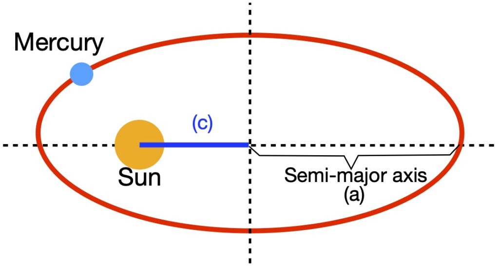
(I use this equation – the result of the second (“easier”) derivation – because the calculations needed to arrive at the advance of the perihelion of Mercury are more intuitive than if the result of the more “difficult” derivation were employed.)
V.A.4 Calculations
We plug the following values into eq. (V.A.42) to arrive at a quantitative answer for the advance of the perihelion of Mercury.


Revolutions per century

V.B Bending of Light
Coming eventually
V.C Gravity Waves
V.C.1 Introduction
Our goal in this section is to show that, when we solve Einstein’s field equation in the case of linearized gravity – in specific coordinate systems – we end up with wave equations. These wave equations represent gravity waves.
We know the general form of the wave equation is:
![\[ v^2 \frac{\partial^2 A}{\partial x^2 } = \frac{\partial^2 A}{\partial t^2 } \]](https://www.samartigliere.com/wp-content/ql-cache/quicklatex.com-70e4be50c3053ffcc59f5717e70565ea_l3.png "Rendered by QuickLaTeX.com")
or
![\[ \frac{\partial^2 A}{\partial x^2 } = \frac{1}{v^2 } \frac{\partial^2 A}{\partial t^2 } \]](https://www.samartigliere.com/wp-content/ql-cache/quicklatex.com-38a61107a928b78ce2d53cfb66c8e09d_l3.png "Rendered by QuickLaTeX.com")
where
is the wave’s amplitude
 is a spatial coordinate
is time
is the wave’s velocity
The classic example of a an entity that obeys the wave equation is electromagnetic radiation. The equations of electromagnetism can be written in several ways:
![\[ \frac{1}{c^2} \frac{\partial^2 E}{\partial t^2} = \frac{\partial^2 E}{\partial x^2} + \frac{\partial^2 E}{\partial y^2} + \frac{\partial^2 E}{\partial z^2}\quad \text{(V.C.1.1)}\]](https://www.samartigliere.com/wp-content/ql-cache/quicklatex.com-ea84a014a36ad5c19fb1738475089f62_l3.png "Rendered by QuickLaTeX.com")
![\[ \frac{\partial^2 E}{\partial (ct)^2} - \frac{\partial^2 E}{\partial x^2} - \frac{\partial^2 E}{\partial y^2} - \frac{\partial^2 E}{\partial z^2} = 0 \quad \text{(V.C.1.2)}\]](https://www.samartigliere.com/wp-content/ql-cache/quicklatex.com-141269c85f49b0d4bac01f0a20459aec_l3.png "Rendered by QuickLaTeX.com")
![\[ \frac{\partial^2 E}{\partial (x^0)^2} - \frac{\partial^2 E}{\partial (x^1)^2} - \frac{\partial^2 E}{\partial (x^2)^2} - \frac{\partial^2 E}{\partial (x^2)^2} = 0 \quad \text{(V.C.1.3)}\]](https://www.samartigliere.com/wp-content/ql-cache/quicklatex.com-b0aae531313044708ffbf0c105710236_l3.png "Rendered by QuickLaTeX.com")
![\[ +\partial_0^2E - \partial_1^2E - \partial_3^2E - \partial_3^2E - 0 \quad \text{(V.C.1.4)} \]](https://www.samartigliere.com/wp-content/ql-cache/quicklatex.com-bcfbebe6f96fd2e485d1523a9d8ce050_l3.png "Rendered by QuickLaTeX.com")
![\[ \eta^{\mu \nu} \partial_{\mu} \partial_{\nu} E = 0 \quad \text{(V.C.1.5)}\]](https://www.samartigliere.com/wp-content/ql-cache/quicklatex.com-65b9630fa50c9d97a01051a61ddc58d0_l3.png "Rendered by QuickLaTeX.com")
![\[ \partial_{\mu} \partial^{\mu} E = 0 \quad \text{(V.C.1.6)}\]](https://www.samartigliere.com/wp-content/ql-cache/quicklatex.com-54aa3aae4fc352bb3ba6c3bba3a98e82_l3.png "Rendered by QuickLaTeX.com")
![\[\square E = 0 \quad \text{where } \square \text{ is the d'Alembert operator} \quad \text{(V.C.1.7)}\]](https://www.samartigliere.com/wp-content/ql-cache/quicklatex.com-deea26569b76587e135535b1c7bf4107_l3.png "Rendered by QuickLaTeX.com")
The equation of gravity waves, on the other hand, are periodic perturbations of the metric of spacetime. They take the following form:

The metric can be written:
![\[ g_ {\mu \nu} + h_ {\mu \nu} \quad \text{(V.C.1.9)}\]](https://www.samartigliere.com/wp-content/ql-cache/quicklatex.com-4f39e7d951d6ae6851a12eb037ed7d13_l3.png "Rendered by QuickLaTeX.com")
where  . It’s actually small perturbations in the
  term that gives us gravity waves. Thus, the equations we derive will actually will be of the form of eq. (V.C.1.8) but with
  replaced by .
V.C.2 Linearized Gravity
V.C.2.a Preliminaries
In the case where gravity is weak, we can approximate the metric by the equation:
![\[ g_{\mu\nu} = \eta _{\mu\nu} + h_{\mu\nu}\quad \|h_{\mu\nu} \ll 1\| \quad \text{(1)}\]](https://www.samartigliere.com/wp-content/ql-cache/quicklatex.com-74f63d0ce817764416e9a706763705f3_l3.png "Rendered by QuickLaTeX.com")
Small perturbations of the  term are responsible for gravity waves.
Recall Einstein’s field equation:
![\[ G_{\mu\nu} \equiv R_{\mu\nu} - \frac12 R g_{\mu\nu} = \frac{8\pi G}{c^4}T_{\mu\nu} \quad \text{(2)} \]](https://www.samartigliere.com/wp-content/ql-cache/quicklatex.com-45b68e17d9835a4e38ea395d6fce85e3_l3.png "Rendered by QuickLaTeX.com")
Our goal, in this section, is to find the  term in Einstein’s field equation under conditions of linearized gravity. To accomplish this, we’ll have to calculate:
- Inverse metric

- Connection Coefficients

- Riemann Tensor

- Ricci Tensor

- Ricci Scalar

Just as a reminder, in linearized gravity:


The inverse metric is given by:
![\[ g_{\mu \sigma} g^{\sigma \nu} = \delta^{\nu}_{\mu} \quad \text{(9)} \]](https://www.samartigliere.com/wp-content/ql-cache/quicklatex.com-d6f95cbd0a3cefb4d14be9dd9560d95b_l3.png "Rendered by QuickLaTeX.com")
and

To see how we get this, click here.

Normally, we would raise and lower indices with  and , respectively. However, since
  is small, we will henceforth raise and lower indices with the Minkowski metric. To see why, click here.

V.C.2.b Connection Coefficients
The general formula for a connection coefficient (or Christoffel symbol) is:
![\[ \Gamma^{\sigma}_{\mu \nu} = \frac 12g^{\sigma \alpha} (\partial_{\nu} g_{\alpha \mu} + \partial_{\mu} g_{\alpha \nu} - \partial_{\alpha} g_{\mu \nu}) \quad \text{(11)} \]](https://www.samartigliere.com/wp-content/ql-cache/quicklatex.com-3f8070356d6137e2b1257247200d062d_l3.png "Rendered by QuickLaTeX.com")
However, in linearized (weak) gravity:
![\[ \partial_{rho} g_{\mu \nu} = \partial_{rho} (\eta_{\mu \nu} + h_{\mu \nu}) = 0 + \partial_{rho} h_{\mu \nu} \quad \text{(12)} \]](https://www.samartigliere.com/wp-content/ql-cache/quicklatex.com-269adb3f2de6b4a79643abe924412001_l3.png "Rendered by QuickLaTeX.com")
So we can replace partial derivatives of with partial derivatives of . Thus:

V.C.2.c Riemann Tensor
Recall from eq. (2.6.38), the Riemann tensor in terms of the connection coefficients is:
![\[ R^{\rho}_{\sigma \mu \nu} = \partial_{\mu} \Gamma^{\rho}_{ \nu \sigma} - \partial_{\nu} \Gamma^{\rho}_{ \mu \sigma} + \Gamma^{\gamma}_{ \nu \sigma} \Gamma^{\rho}_{ \mu \gamma} - \Gamma^{\delta}_{ \mu \sigma} \Gamma^{\rho}_{ \nu \delta} \quad \text{(14)} \]](https://www.samartigliere.com/wp-content/ql-cache/quicklatex.com-04f62e6b0af682f8983c638021f3e7b7_l3.png "Rendered by QuickLaTeX.com")
The connection coefficients in linearized gravity are:
![\[ \Gamma_{\nu \sigma}^\gamma=\frac{1}{2} \eta^{\gamma \alpha}\left(\partial_\sigma h_{\alpha \nu}+\partial_v h_{\alpha \sigma}-\partial_\alpha h_{\nu \sigma}\right) \]](https://www.samartigliere.com/wp-content/ql-cache/quicklatex.com-61dbd760bf6f664493dca8e7a013f920_l3.png "Rendered by QuickLaTeX.com")
![\[ \Gamma_{\mu \gamma}^\rho=\frac{1}{2} \eta^{\rho \alpha}\left(\partial_\gamma h_{\alpha \mu}+\partial_\mu h_{\alpha \gamma}-\partial_\alpha h_{\mu \gamma}\right) \]](https://www.samartigliere.com/wp-content/ql-cache/quicklatex.com-3592de5cfb3f12a6286a988678a0aced_l3.png "Rendered by QuickLaTeX.com")
The  terms yield results like this:

All of the  terms between the parentheses are negligible. Thus, the terms in the expression for the Riemann tensor are zero. Eq. (14), then, becomes:
![\[ R^{\rho}_{\sigma \mu \nu} \approx \partial_{\mu} \Gamma^{\rho}_{ \nu \sigma} - \partial_{\nu} \Gamma^{\rho}_{ \mu \sigma} \quad \text{(15)} \]](https://www.samartigliere.com/wp-content/ql-cache/quicklatex.com-9f32d2431efe1387249ef7b03a2c64a8_l3.png "Rendered by QuickLaTeX.com")
We substitute in the values for the connection coefficients into eq. (15) and rearrange. That gives us:

V.C.2.d Ricci Tensor
To get the Ricci tensor from the Riemann tensor, we simply contract the Riemann tensor in its third index:
![\[ R_{\sigma \nu} = R^{\mu}_{\sigma \mu \nu} \quad \text{(17)} \]](https://www.samartigliere.com/wp-content/ql-cache/quicklatex.com-4e0218c5050c50029eb38570532c1963_l3.png "Rendered by QuickLaTeX.com")
![\[ R_{\sigma \mu \nu}^\mu=\frac{1}{2} \eta^{\mu \alpha}\left(\partial_\mu \partial_\sigma h_{\alpha \nu}-\partial_\mu \partial_\alpha h_{\nu \sigma}-\partial_v \partial_\sigma h_{\alpha \mu}+\partial_v \partial_\alpha h_{\mu \sigma}\right) \quad \text{(18)} \]](https://www.samartigliere.com/wp-content/ql-cache/quicklatex.com-a0725a029cba549941da757524046d0f_l3.png "Rendered by QuickLaTeX.com")
The superscript on the  term raises som indices:
![\[R_{\sigma v}=\frac{1}{2}\left(\partial_\mu \partial_\sigma h_\nu^\mu-\partial^\mu \partial_\mu h_{\nu \sigma}-\partial_v \partial_\sigma h_\mu^\mu+\partial_v \partial_\alpha h_\sigma^\alpha\right) \quad \text{(19)} \]](https://www.samartigliere.com/wp-content/ql-cache/quicklatex.com-f69df23bbf534984720a9b3b2ca8d0f1_l3.png "Rendered by QuickLaTeX.com")
Next, we define the scalar  and plug this into eq. (19). We could also place the d’Alembert operator (
 ) for
) for  , but for ensuing calculations, I think this will just make things more confusing. So I won’t make that substitution here. At any rate, we have – for the Ricci tensor – the following equation:
![\[R_{\sigma v}=\frac{1}{2}\left(\partial_\mu \partial_\sigma h_v^\mu+\partial_v \partial_\alpha h_\sigma^\alpha-\partial^{\mu}\partial_{\mu} h_{v \sigma}-\partial_v \partial_\sigma h\right) \quad \text{(20)} \]](https://www.samartigliere.com/wp-content/ql-cache/quicklatex.com-00e58aa1abe71e4ffbcb61ec5ccb5a35_l3.png "Rendered by QuickLaTeX.com")
V.C.2.e Ricci Scalar
We create the Ricci Scalar by contracting the Ricci Tensor:

We make the following change in repeated variables in the second term within parentheses in eq. (21) ( ):
):

Since is symmetric,  . Therefore, we have:

V.C.2.f Einstein Tensor
Now that we have expressions for the Ricci tensor, the Ricci scalar and the metric, we can find an expression for the Einstein tensor.

We’d like to convert eq. (23) into a form that will be more convenient for future manipulations. To do this, we need to use that following mathematical trick. For repeated indices in the partial derivative and metric correction term , we can raise the partial derivative’s index and lower the metric correction term index, as follows:
![\[ h^{\mu \nu} = \eta^{\mu \alpha} h_{\alpha}^{\nu} \]](https://www.samartigliere.com/wp-content/ql-cache/quicklatex.com-5db98c85b1b3d19a77cf1563ae05c15f_l3.png "Rendered by QuickLaTeX.com")
![\[ \partial_{\mu} h^{\mu \nu} = \partial_{\mu} \eta^{\mu \alpha} h_{\alpha}^{\nu} \]](https://www.samartigliere.com/wp-content/ql-cache/quicklatex.com-bf601b7e8dad668b6a1720a814d1033a_l3.png "Rendered by QuickLaTeX.com")
![\[ \partial_{\mu} h^{\mu \nu} = \partial^\alpha h_{\alpha}^{\nu}\quad \text{(24)}\]](https://www.samartigliere.com/wp-content/ql-cache/quicklatex.com-c48fb67f7bccf26b260a47d50c221676_l3.png "Rendered by QuickLaTeX.com")
Using this technique on eq. (23), we obtain:

We now make the following change of variables:
![\[\overline{h} \equiv h_{\mu \nu} - \frac12 \eta _{\mu \nu} h \quad \text{(26)}\]](https://www.samartigliere.com/wp-content/ql-cache/quicklatex.com-2c13dd3c7fd2c6f0b25ff4a34c533a90_l3.png "Rendered by QuickLaTeX.com")
![\[h_{\mu \nu} = \overline{h} + \frac12 \eta _{\mu \nu} h \quad \text{(27)}\]](https://www.samartigliere.com/wp-content/ql-cache/quicklatex.com-b2d1aceb387509cdd5840e54ea14fad2_l3.png "Rendered by QuickLaTeX.com")
We replace the values of the terms in eq. (25) with the value on the righthand side of eq. (27), giving us:
![\[G_{\mu \nu}=\frac{1}{2}\left(\partial^\alpha \partial_\mu \bar{h}_{\alpha \nu}+\partial^\alpha \partial_\nu \bar{h}_{\mu \alpha}-\partial^\alpha \partial_\alpha \bar{h}_{\mu \nu}-\eta_{\mu \nu} \partial^\alpha \partial^\beta \bar{h}_{\alpha \beta}\right)\quad \text{(28)}\]](https://www.samartigliere.com/wp-content/ql-cache/quicklatex.com-9d4b513eed60cba5994f644a65db4ae7_l3.png "Rendered by QuickLaTeX.com")
Figure 1 shows how we get from eq. (25) to eq. (28).
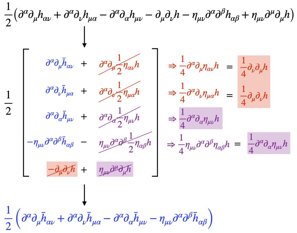
Lorenz Gauge
In the last section, we found an equation for the Einstein tensor in terms of a variable that reflects small perturbations of the metric . Specifically:
where
![\[ g_{\mu \nu} = \eta_{\mu \nu} + h_{\mu \nu} \]](https://www.samartigliere.com/wp-content/ql-cache/quicklatex.com-f22de9dabfe2316082f0eab8077b4791_l3.png "Rendered by QuickLaTeX.com")
and
![\[h_{\mu \nu} = \overline{h} + \frac12 \eta _{\mu \nu} h \]](https://www.samartigliere.com/wp-content/ql-cache/quicklatex.com-8ab4e49f3d3eeecfda651dd3f050a82b_l3.png "Rendered by QuickLaTeX.com")
Our ultimate goal, though, is to get a wave equation from eq. (28). It turns out that we can do a change of coordinates such that all of the terms on the right side of eq. (28) equal zero except  equal zero:
![\[G_{\mu \nu}=\frac{1}{2}\left(\underbrace{\cancel{\partial^\alpha \partial_\mu \bar{h}_{\alpha \nu}}}_{0}+\underbrace{\cancel{\partial^\alpha \partial_\nu \bar{h}_{\mu \alpha}}}_{0}-\partial^\alpha \partial_\alpha \bar{h}_{\mu \nu}-\underbrace{\cancel{\eta_{\mu \nu} \partial^\alpha \partial^\beta \bar{h}_{\alpha \beta}}}_{0}\right)}\right)\quad \text{(V.C.3.1)}\]](https://www.samartigliere.com/wp-content/ql-cache/quicklatex.com-f85227cfeca302318b2d0bde418f30e8_l3.png "Rendered by QuickLaTeX.com")
In the vacuum (i.e.,  ), eq. (V.C.3.1) becomes:
![\[ \partial^\alpha \partial_\alpha \bar{h}_{\mu \nu} = 0\quad \text{(V.C.3.2)}\]](https://www.samartigliere.com/wp-content/ql-cache/quicklatex.com-f26af9b9356087feb2013a27221fe2c0_l3.png "Rendered by QuickLaTeX.com")
The solution to eq. (V.C.3.2) is a wave, which is what we want. Our task now is to find the coordinate change(s) that bring about the above conditions. Such a coordinate system is called a Lorenz gauge.
It so happens that, if  then the 3 terms in eq. (28) that we want to become zero, actually become zero. So let’s see if we can manipulate eq. (28) such that this occurs. Recall from eq. (24) that:
We’ll apply this to the terms in eq. (28) we wish to negate and see if we can get rid of them. We’ll start with the 4th term on the righthand side of eq. (28)  . We’ll work on the
  part:
part:

So the 4th term becomes zero.
Next, we’ll attack the 1rst term on the righthand side,  .
.

So the 1rst term goes to zero, too.
Finally, we manipulate the 2nd term  . We get:

The 2nd term vanishes as well.
Now what we need to do is find a coordinate system(s) that makes .
The coordinate transformation we’ll make is called a displacement field:
![\[ \widetilde{x}^{\alpha} = x^{\alpha} + \xi^{\alpha} \quad \|\xi^{\alpha} \| \ll 1 \quad \text{(V.C.3.3)} \]](https://www.samartigliere.com/wp-content/ql-cache/quicklatex.com-4531612a34b5e53ac0f9fc6474ec9921_l3.png "Rendered by QuickLaTeX.com")
where
 are the old coordinates, i.e., (ct, x, y, z)
 are the new coordinates
 are the components of the displacement field
The displacement field is a tiny vector added to each point in space. The result is a new coordinate system (Figure V.C.3.1):
eigenchris. Relativity 109c: Gravitational Waves – Wave Derivation (The Lorenz Gauge).Feb 7, 2022
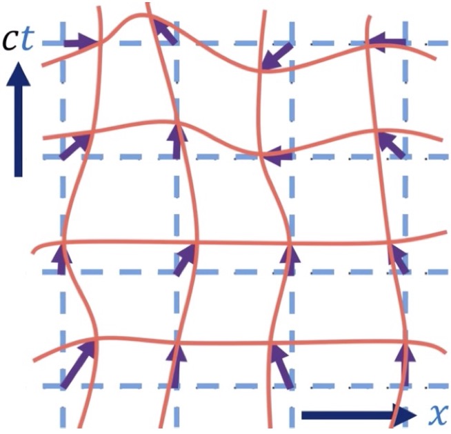
In the diagram, the blue dotted lines represent the original coordinates. The small purple vectors represent the displacement field. And the curved orange lines represent the new coordinate axes associated with the displacement field.
So we have:
![\[ \widetilde{x}^{\alpha} = x^{\alpha} + \xi^{\alpha} \quad \text{(V.C.3.3)} \]](https://www.samartigliere.com/wp-content/ql-cache/quicklatex.com-7c64e43b34de43cbe2fc65240cea4ed7_l3.png "Rendered by QuickLaTeX.com")
![\[ x^{\alpha} = \widetilde{x}^{\alpha} - \xi^{\alpha} \quad \text{(V.C.3.4)} \]](https://www.samartigliere.com/wp-content/ql-cache/quicklatex.com-f5d8d15b7d865f4da1a78726e4d8f5d1_l3.png "Rendered by QuickLaTeX.com")
We differentiate eq. (33) and eq. (34) and get:
![\[ \frac{\partial \widetilde{x}^{\alpha}}{\partial x^{\beta}} = \frac{\partial x^{\alpha}}{\partial x^{\beta}} + \frac{\partial \xi^{\alpha}}{\partial x^{\beta}} = \delta^{\alpha}_{\beta} + \frac{\partial \xi^{\alpha}}{\partial x^{\beta}} \quad \text{(V.C.3.5)} \]](https://www.samartigliere.com/wp-content/ql-cache/quicklatex.com-4833463e102622bf2a347c07c5427937_l3.png "Rendered by QuickLaTeX.com")
![\[ \frac{\partial x^{\alpha}}{\partial \widetilde{x}^{\beta}} = \frac{\partial \widetilde{x}^{\alpha}}{\partial \widetilde{x}^{\beta}} - \frac{\partial \xi^{\alpha}}{\partial \widetilde{x}^{\beta}} = \delta^{\alpha}_{\beta} - \frac{\partial \xi^{\alpha}}{\partial x^{\sigma}}\frac{\partial x^{\sigma}}{\partial \widetilde{x}^{\beta}} \quad \text{(V.C.3.6)} \]](https://www.samartigliere.com/wp-content/ql-cache/quicklatex.com-cd53c31896a82c8347d0154d5bda536e_l3.png "Rendered by QuickLaTeX.com")
Next, we take the indices on the non-expanded term on the righthand side of eq. (V.C.3.6) and relabel them as . That gives us:
![\[ \frac{\partial x^{\sigma}}{\partial \widetilde{x}^{\beta}} = \delta^{\sigma}_{\beta} - \frac{\partial \xi^{\sigma}}{\partial \widetilde{x}^{\beta}} \quad \text{(V.C.3.7)} \]](https://www.samartigliere.com/wp-content/ql-cache/quicklatex.com-630f8dcae94dae0ed7e19171c972bc2a_l3.png "Rendered by QuickLaTeX.com")
Then we substitute the value of  into the rightmost term of eq. (V.C.3.6) yielding:

Since  and its derivatives are very small, the product of 2 derivatives of is negligible and we can ignore it. We can use
  to change the lower index on the term to its left, to . We get:
![\[ \frac{\partial x^\alpha}{\partial \widetilde{x}^\beta}=\delta_\beta^\alpha-\frac{\partial \xi^\alpha}{\partial x^\beta} \quad \text{(V.C.3.9)} \]](https://www.samartigliere.com/wp-content/ql-cache/quicklatex.com-36b6c8fb46a3fc2805505cad0fe25b4f_l3.png "Rendered by QuickLaTeX.com")
The metric changes under a change of coordinates, as follows:
![\[ \widetilde{g}_{\alpha \beta} = \frac{\partial x^{\mu}}{\partial \widetilde{x}^{\alpha}}\frac{\partial x^{\nu}}{\partial \widetilde{x}^{\beta}} g_{\mu \nu} \quad \text{(V.C.3.10)} \]](https://www.samartigliere.com/wp-content/ql-cache/quicklatex.com-3ae1ee19ef5853f25ac14e3f06b1f6bd_l3.png "Rendered by QuickLaTeX.com")
We plug the results of eq. (V.C.3.9), and substitute the expanded version of the metric  , into eq. (V .C.3.10). That gives us:

To save space, we’ll use comma notation to indicate derivatives (e.g.,  . We institute this comma notation, distribute terms and use the Minkowski metric to lower some indices. We also note that
  . Eq. (V.C.3.11) becomes:

Recognizing that:
![\[ g_{\alpha \beta} = \eta_{\alpha \beta} +h_{\alpha \beta} \]](https://www.samartigliere.com/wp-content/ql-cache/quicklatex.com-65eca28760af328ba8e2d190d0cce7f0_l3.png "Rendered by QuickLaTeX.com")
and
![\[ \widetilde{g}_{\alpha \beta} = \eta_{\alpha \beta} +\[ g_{\alpha \beta} = \eta_{\alpha \beta} + \widetilde{h}_{\alpha \beta} \]](https://www.samartigliere.com/wp-content/ql-cache/quicklatex.com-fd58d4e67dad71d483cebdb16dc0ec68_l3.png "Rendered by QuickLaTeX.com")
we can transform eq. (V.C.3.12) into:

As an aside, it turns out that the components of the Riemann curvature tensor don’t change under a coordinate change created by a small displacement field:
![\[\widetilde{R}^{\rho}_{\sigma \mu \nu} = R^{\rho}_{\sigma \mu \nu}\quad \text{(V.C.3.14)}\]](https://www.samartigliere.com/wp-content/ql-cache/quicklatex.com-0fe39f9f77f03acca6024907c26fce59_l3.png "Rendered by QuickLaTeX.com")
Proof of this can be found in the eigenchris YouTube video, Relativity 109c: Gravitational Waves – Wave Derivation (The Lorenz Gauge) at 10:30.
At any rate, recall that our goal is for our change  leads to the change
  such that
  i.e., the Lorenz condition.
We know that:
![\[ \widetilde{h}_{\mu \nu} &\equiv h_{\mu \nu}-\xi_{\mu, \nu}-\xi_{\nu, \mu}\quad \text{(V.C.3.15)} \]](https://www.samartigliere.com/wp-content/ql-cache/quicklatex.com-d5650022fdf99d957dd7d054906bd1ba_l3.png "Rendered by QuickLaTeX.com")
Therefore:
![\begin{align*} \overline{\widetilde{h}}_{\mu \nu} &\equiv \widetilde{h}_{\mu \nu}-\frac{1}{2} \eta_{\mu \nu} \widetilde{h}= \widetilde{h}_{\mu \nu} - \frac12\eta_{\mu \nu}\eta^{\alpha \beta}\widetilde{h}_{\alpha \beta} \\ \overline{\widetilde{h}}_{\mu \nu}&=\left(h_{\mu \nu}-\xi_{\mu, \nu}-\xi_{\nu, \mu}\right)-\frac{1}{2} \eta_{\mu \nu}\left[\eta^{\alpha \beta}\left(h_{\alpha \beta}-\xi_{\alpha, \beta}-\xi_{\beta, \alpha}\right)\right]\\ &=h_{\mu \nu}-\frac{1}{2} \eta_{\mu \nu} h-\xi_{\mu, \nu}-\xi_{\nu, \mu}+\frac{1}{2} \eta_{\mu \nu} \eta^{\alpha \beta} \xi_{\alpha, \beta}+\frac{1}{2} \eta_{\mu \nu} \eta^{\alpha \beta} \xi_{\beta, \alpha} \\ &=h_{\mu \nu}-\frac{1}{2} \eta_{\mu \nu} h-\xi_{\mu, \nu}-\xi_{\nu, \mu}+\frac{1}{2} \eta_{\mu \nu} \xi_{, \beta}^\beta+\frac{1}{2} \eta_{\mu \nu} \xi_{, \beta}^\beta \\ \eta^{\mu \alpha} \eta^{\nu \beta} \overline{\widetilde{h}}_{\mu \nu}&=\eta^{\mu \alpha} \eta^{\nu \beta}\left(\overline{h}_{\mu \nu}-\xi_{\mu, \nu}-\xi_{\nu, \mu}+\eta_{\mu \nu} \xi^\sigma, \sigma\right) \\ \overline{h}^{\alpha \beta}&=\overline{h}^{\alpha \beta}-\eta^{\mu \alpha} \eta^{\nu \beta} \xi_{\mu, v}-\eta^{\mu \alpha} \eta^{\nu \beta} \xi_{\nu, \mu}+\eta^{\alpha \beta} \xi_{, \sigma}^\sigma \\ \overline{\tilde{h}}^{\alpha \beta}&=\overline{h^{\alpha \beta}}-\eta^{\nu \beta} \xi^\alpha{ }_{, \nu}-\eta^{\mu \alpha} \xi_{, \mu}^\beta+\eta^{\alpha \beta} \xi_{, \sigma}^\sigma \\ \overline{\tilde{h}}^{\alpha \beta}&=\overline{h_{, \beta}^{\alpha \beta}}-\eta^{\nu \beta} \xi_{, \nu \beta}^\alpha-\eta^{\mu \alpha} \xi_{, \mu \beta}^\beta+\eta^{\alpha \beta} \xi_{, \sigma \beta}^\sigma \\ \beta \rightarrow \mu &\text{ and } \sigma \rightarrow \beta \text{ for rightmost term} \\ \overline{\tilde{h}}^{\alpha \beta}&=\overline{h_{, \beta}^{\alpha \beta}}-\eta^{\nu \beta} \xi_{, \nu \beta}^\alpha-\cancel{\eta^{\mu \alpha} \xi_{, \mu \beta}^\beta}+\cancel{\eta^{\alpha \mu} \xi_{,\beta \mu}^{\beta}} \\ \overline{\tilde{h}}^{\alpha \beta}&=\overline{h}_{, \beta}^{\alpha \beta}-\eta^{\nu \beta} \partial_{\nu} \partial_{\beta}\xi^\alpha \\ \partial_{\beta}\,\overline{\tilde{h}}^{\alpha \beta}&=\partial_{\beta}\,\overline{h}^{\alpha \beta}- \partial^{\beta} \partial_{\beta}\xi^\alpha \\ \partial_{\beta}\,\overline{\tilde{h}}^{\alpha \beta}&=\partial_{\beta}\,\overline{h}^{\alpha \beta}- \square\xi^\alpha \quad \text{(V.C.3.16)}\end{align*}](https://www.samartigliere.com/wp-content/ql-cache/quicklatex.com-dd901b6c02652d67cb6b18ecc6bbdc14_l3.png "Rendered by QuickLaTeX.com")
If we choose such that  , then
  which, of course, is the Lorenz condition.
Not that the choice of is not unique. If we have  such that
  , then this will also satisfy the Lorenz condition since:
![\[ \partial_{\beta}\,\overline{\tilde{h}}^{\alpha \beta} = \square(\xi^{\alpha} + \chi^{\alpha}) = \square \xi^{\alpha} + \underbrace{\square \chi^{\alpha}}_{0} = \square \xi^{\alpha} \quad \text{(V.C.3.17)} \]](https://www.samartigliere.com/wp-content/ql-cache/quicklatex.com-4f797a4bcba820a86d31ea742c55225d_l3.png "Rendered by QuickLaTeX.com")
Thus, the Lorenz gauge is a whole class of coordinates changes that satisfy the Lorenz condition.
So, if we find a Lorenz gauge, then:
![\[\partial_{\beta}\,\overline{\tilde{h}}^{\alpha \beta} = \partial^{\beta}\,\overline{\tilde{h}}_{\alpha \beta} = 0\]](https://www.samartigliere.com/wp-content/ql-cache/quicklatex.com-26694eac18b782ca891f0d5a9809358f_l3.png "Rendered by QuickLaTeX.com")
and
![\[ \widetilde{G}_{\mu \nu}=\frac{1}{2}\left(\underbrace{\cancel{\partial^\alpha \partial_\mu \overline{\widetilde{h}}_{\alpha \nu}}}_{0}+\underbrace{\cancel{\partial^\alpha \partial_\nu \overline{\widetilde{h}}_{\mu \alpha}}}_{0}-\underbrace{\cancel{\eta_{\mu \nu} \partial^\alpha \partial^\beta \overline{\widetilde{h}}_{\alpha \beta}}}_{0}-\partial^\alpha \partial_\alpha \overline{\widetilde{h}}_{\mu \nu}\right) \quad \text{(V.C.3.18)} \]](https://www.samartigliere.com/wp-content/ql-cache/quicklatex.com-49dc90cbba1c02bc065a6188c5443ff2_l3.png "Rendered by QuickLaTeX.com")
In linearized gravity and the Lorenz gauge:
![\[ \widetilde{G}_{\mu \nu} = \frac12 \square \overline{\widetilde{h}}_{\mu \nu} = \frac{8 \pi G}{c^4}\,\widetilde{T}_{\mu \nu} \quad \text{(V.C.3.19)} \]](https://www.samartigliere.com/wp-content/ql-cache/quicklatex.com-8d9f0fd3f2c95e217ba9044e9bc3f8ef_l3.png "Rendered by QuickLaTeX.com")
If we’re in a vacuum,  , which means that:
![\[ \square \overline{\widetilde{h}}_{\mu \nu} = 0 \quad \text{(V.C.3.20)} \]](https://www.samartigliere.com/wp-content/ql-cache/quicklatex.com-03c9a6bda280f88e006ef2c67908568b_l3.png "Rendered by QuickLaTeX.com")
And, of course, eq. (V.C.3.20) is a wave equation, which is what we were trying to show.